
AP Syllabus focus:
‘Use difference quotients like [f(b) − f(a)] / (b − a) to compute the average rate of change of a function over an interval using formulas, tables, or graphs.’
Understanding average rate of change helps reveal how a function behaves across an interval by comparing output differences to input differences using graphical or tabular representations.
Understanding Average Rate of Change
The average rate of change of a function over an interval provides a numerical measure of how the function’s output varies relative to changes in the input. When presented with graphs or tables, students analyze visual or numerical information to determine this relationship. Because this topic focuses strictly on graphical and tabular contexts, attention centers on reading values, interpreting changes, and applying structured difference quotients.
Average Rate of Change: The change in a function’s output divided by the change in its input over an interval .
This idea generalizes the notion of a secant line, which represents the line connecting two points on a graph and captures the function’s behavior between them.
The Difference Quotient Structure
To compute an average rate of change, AP Calculus AB emphasizes the difference quotient, a structured expression comparing output and input changes. The specification explicitly references formulas of the type because this captures the essential relationship between two points on a function.
= Change in the function’s output
= Change in input across the interval
Students must be able to recognize this structure when information is extracted from graphs or from tables of values. This reinforces the interpretation that the function’s behavior between and is summarized by a single value expressing overall trend.
A secant line’s slope is numerically equal to this difference quotient, which emphasizes the geometric meaning behind the computation.
Using Graphs to Determine Average Rate of Change
Graphs provide a visual representation of how a function behaves over an interval, allowing students to locate key coordinate pairs and compute difference quotients. Careful interpretation ensures accuracy even when the graph is not drawn to scale.
From a graph, the average rate of change on an interval [a, b] is the slope of the secant line joining the points (a, f(a)) and (b, f(b)).
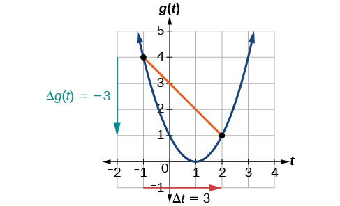
This graph shows two points on a function joined by a secant line, with horizontal and vertical arrows illustrating changes in input and output. The image highlights how the slope of this line represents the average rate of change across the interval. It visually connects the difference quotient to geometric slope. Source.
Key Considerations When Working from Graphs
Identify exact or estimated coordinates at and .
Read corresponding -values directly from the graph or from labels.
Apply the difference quotient using the identified function values.
Interpret the result in terms of increasing or decreasing behavior.
When analyzing graphs, students should focus on whether the function rises or falls between the chosen points and how steeply this change occurs. Because graphs may not show numerical precision, approximations may be necessary, but the structural reasoning remains consistent. The process reinforces the connection between geometric slope and numeric rate of change.
Using Tables to Determine Average Rate of Change
Tables present discrete pairs of input and output values, enabling direct substitution into the difference quotient formula. Students must read entries carefully to ensure the correct values are used for each endpoint.
Key Considerations When Working from Tables
Locate the row containing and note its function value.
Locate the row containing and record its function value.
Compute the difference in -values to understand output change.
Divide by the difference in -values to obtain the average rate of change.
Where tables provide evenly spaced inputs, the difference quotient often simplifies conceptual reasoning. However, the interpretation remains the same: the result expresses how much the function changes per unit change in the input.
Interpreting the Meaning of the Average Rate of Change
Interpreting the average rate of change is crucial because the value is not merely computational—it conveys how the underlying quantity behaves across an interval. Students should connect the numerical value to the graph’s shape or table’s data pattern and describe the behavior of the function over the designated range.
Important Interpretive Points
A positive value indicates that the function’s output increases as the input increases.
A negative value indicates decreasing behavior across the interval.
A large magnitude suggests steep change, while a small magnitude suggests gradual change.
The value summarizes overall behavior and may not represent behavior at individual points.
This interpretive component ties directly to the AP emphasis on conceptual understanding rather than solely procedural calculation. Students must use the computed value to articulate how the function behaves in context, whether graphical or numerical.
Processes for Computing from Graphs or Tables
Identify the interval endpoints clearly.
Extract or estimate and from the provided representation.
Substitute values into the difference quotient.
State the result in appropriate descriptive terms.
Connect the value to observable behavior in the graph or numerical trends in the table.
In real data, a table of measurements and the graph of those points describe the same function, so the average rate of change over an interval can be interpreted consistently from either representation.
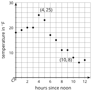
This scatter plot displays temperature values at hourly intervals, illustrating how both the table and the graph represent the same underlying function. Average rates of change can be analyzed by comparing temperature differences across selected intervals. Some intervals shown extend beyond those emphasized in the syllabus, but all reinforce the interpretation of average rate of change. Source.
The AP syllabus emphasizes that students should be comfortable performing these steps regardless of representation because the ideas underpin foundational concepts in later derivative topics. Understanding this average rate of change prepares students for recognizing how instantaneous rates emerge from shrinking intervals, though such development belongs to later subsubtopics.
Practice Questions
The graph of a function f shows two points: A at x = 1 with f(1) = 4, and B at x = 5 with f(5) = 12.
Find the average rate of change of f on the interval [1, 5].
(1–3 marks)
Question 1 (1–3 marks)
Correct substitution into the average rate of change formula: (12 − 4) / (5 − 1) (1 mark)
Correct numerical value: 8 / 4 = 2 (1 mark)
Correct units or appropriate interpretation if given (e.g., "the function increases by 2 units per x-unit") (1 mark)
The table below shows values of a differentiable function g.
x: 0 2 4 6
g(x): 5 9 14 10
(a) Estimate the average rate of change of g on the interval [0, 4].
(b) Estimate the average rate of change of g on the interval [4, 6].
(c) Using your results, comment on how the behaviour of g changes over these intervals.
(4–6 marks)
Question 2 (4–6 marks)
(a)
Correct difference in outputs: 14 − 5 = 9 (1 mark)
Correct difference in inputs: 4 − 0 = 4 (1 mark)
Correct average rate of change: 9 / 4 = 2.25 (1 mark)
(b)
Correct difference in outputs: 10 − 14 = −4 (1 mark)
Correct difference in inputs: 6 − 4 = 2 (1 mark)
Correct average rate of change: −4 / 2 = −2 (1 mark)
(c)
Clear statement comparing interval behaviours:
For example, “g is increasing on [0, 4] but decreasing on [4, 6], as shown by positive then negative average rates of change.” (1 mark)
FAQ
Accuracy depends on how clearly the graph is scaled. Small plotting or reading errors have limited impact if the interval is large, but they matter more on short intervals.
To improve accuracy:
• Use gridlines whenever possible.
• Identify exact intercepts or labelled points before estimating.
• Avoid relying on curvature; only the coordinates of the interval endpoints matter.
Small vertical differences between two functions can accumulate over a long interval, meaning visually similar graphs may nevertheless show different rates of change.
Differences also arise if one graph has gentle curvature while another has more pronounced bending between the same endpoints, altering the secant line’s slope.
Yes, this occurs when the slope of the secant line matches the slope of the tangent line at some point in the interval.
This situation aligns with the Mean Value Theorem (though not required knowledge at this stage), which guarantees such a point for differentiable functions on closed intervals.
The value is especially sensitive when the function:
• has steep curvature,
• changes direction frequently,
• or contains rapid fluctuations in output.
Short intervals magnify local behaviour, while long intervals smooth out these variations.
A table is sufficient if the endpoints of the interval appear explicitly; intermediate points are helpful but not required.
However, reliability improves when:
• the table entries are precise rather than rounded,
• the interval is not extremely narrow,
• and the function behaves smoothly rather than oscillating sharply between recorded values.
