
AP Syllabus focus:
‘Define the instantaneous rate of change at x = a as the limit of a difference quotient, such as lim₍h→0₎ [f(a + h) − f(a)] / h, when this limit exists.’
Instantaneous rate of change describes how a quantity varies at an exact moment. It is defined using limits, connecting average changes over intervals to precise, point-based behavior.
Understanding Instantaneous Rate of Change
The instantaneous rate of change of a function at a point captures how rapidly the function’s output changes with respect to its input at a specific value. This idea refines the concept of average change by imagining intervals shrinking toward a single point.
Instantaneous Rate of Change: The value that represents how a function changes at an exact input, defined as the limit of a difference quotient as the interval approaches zero.
To appreciate this concept, it is helpful to contrast it with the average rate of change computed over a finite interval. Whereas an average rate summarizes change over space or time, the instantaneous rate focuses on the precise behavior of the function at one location on its graph.
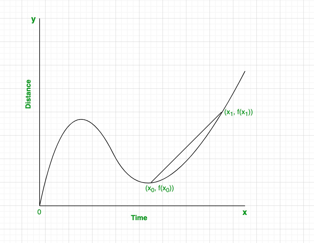
A curve shows two points connected by a secant line, whose slope represents the average rate of change between x0x_0x0 and x1x_1x1. The labeled time–distance context provides a concrete interpretation but extends beyond the formal AP definition. The secant line contrasts with the tangent-line-based instantaneous rate of change. Source.
The Difference Quotient Framework
The central tool for defining instantaneous change is the difference quotient, which compares the change in output to the change in input over an interval. As the interval becomes very small, this quotient approaches a limiting value when it exists.
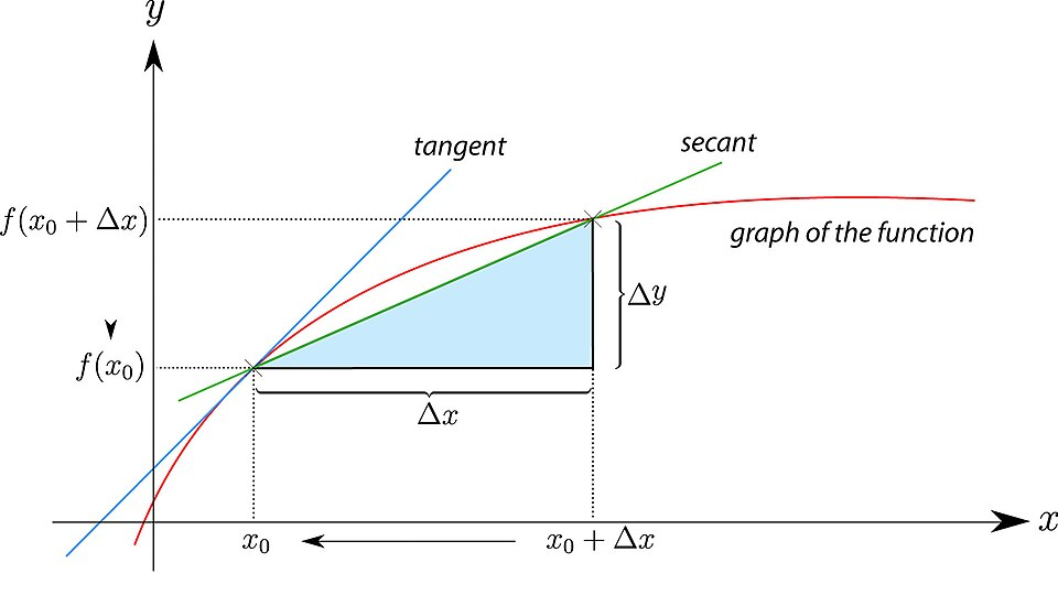
The diagram displays secant and tangent lines on a curve, showing how the slope ΔyΔx\frac{\Delta y}{\Delta x}ΔxΔy approaches the instantaneous rate of change as Δx→0\Delta x \to 0Δx→0. The highlighted Δx\Delta xΔx–Δy\Delta yΔy rectangle is an additional visual aid beyond the AP requirements. Source.
= Change in the function’s output
= Change in the input, representing an increasingly small interval
This limiting value represents the slope of the curve at . When the limit exists, it defines the derivative, linking this subtopic directly to the formal development of differentiation. Between such conceptual and graphical interpretations, the limit-based definition remains foundational.
A function’s ability to produce a meaningful instantaneous rate of change depends on its behavior at the point of interest. Functions with smooth graphs typically produce a finite limit, while functions with sharp corners, discontinuities, or vertical tangent behavior may not.
Why the Limit Process Matters
The use of limits ensures that the instantaneous rate of change is not guessed but rigorously defined. Shrinking the interval between and allows the average rate of change to approach a single, stable value.
Key conceptual roles of the limit process include:
Allowing transition from secant line slopes to a tangent line slope, representing the curve’s direction at one point.
Ensuring that the resulting rate of change is independent of interval size once the limit is considered.
Providing a consistent method that applies across algebraic, graphical, and contextual representations.
When this limit exists, we say the function is differentiable at , and the instantaneous rate of change equals its derivative. When the limit fails to exist, the function lacks an instantaneous rate of change at that point.
Interpreting the Instantaneous Rate in Context
In applied settings, the instantaneous rate of change provides deep insight into how real quantities evolve. Interpreting this value requires connecting the mathematical definition to the meaning of the variables.
Common contextual interpretations include:
In motion problems, the instantaneous rate of change of position represents velocity.
In growth models, it may represent the momentary growth rate of a population or quantity.
In economics, it can describe the marginal change of cost, revenue, or profit at a specific production level.
These interpretations rest on treating the function’s derivative at as the best local linear approximation of change. The limit-based definition ensures that this approximation is mathematically justified.
Graphical Meaning of the Instantaneous Rate of Change
Graphically, the instantaneous rate of change corresponds to the slope of the tangent line to the curve at a point.
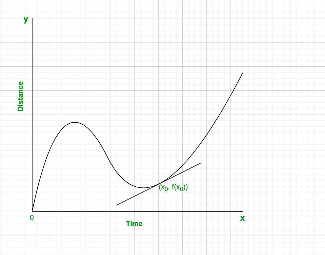
The tangent line touches the curve at (x0,f(x0))(x_0, f(x_0))(x0,f(x0)), showing the slope that represents the instantaneous rate of change at that point. The labeled time–distance setting is contextual rather than required by the AP definition. Source.
Imagining or sketching the tangent line helps reveal how steeply the function is increasing or decreasing at that location.
Important graphical insights:
A positive instantaneous rate of change indicates that the function is rising at that point.
A negative value shows that the function is falling at that point.
A value of zero corresponds to a horizontal tangent, often signaling a local maximum, minimum, or point of inflection in more complex analyses.
The tangent line’s slope provides a visual representation of the limit definition, making the abstract concept more intuitive.
Structural Requirements for the Limit to Exist
The existence of the instantaneous rate of change relies on stable behavior near . If the function oscillates too wildly, exhibits a sharp corner, or is not defined in a small neighborhood around the point, then the limit of the difference quotient may not exist.
To ensure existence, the function should:
Display predictable, smooth behavior near the input value.
Avoid abrupt directional changes that create inconsistent secant slopes.
Be defined on an interval that includes points arbitrarily close to .
Recognizing these restrictions deepens understanding of when the limit-based definition meaningfully applies.
Practice Questions
Question 1 (1–3 marks)
A function f is defined for all real numbers, and its values near x = 2 are shown in the table below:
x: 1.9 , 2.0 , 2.1
f(x): 4.2 , 4.5 , 4.9
(a) Use the table to estimate the instantaneous rate of change of f at x = 2.
(b) State whether your estimate is likely to be an overestimate or an underestimate, giving a brief reason.
Question 1 (Total: 3 marks)
(a)
• 1 mark for computing a valid difference quotient using values near x = 2.
(For example: (4.9 − 4.5) / (2.1 − 2.0) = 4, or (4.5 − 4.2) / (2.0 − 1.9) = 3.)
• 1 mark for stating a reasonable estimate for the instantaneous rate of change, typically midway or justified by symmetry (e.g., approximately 3.5–4).
(b)
• 1 mark for a correct statement such as “The estimate is likely an overestimate because the function appears increasing at an increasing rate,” or an equivalent justified comment based on the table.
Question 2 (4–6 marks)
A differentiable function g satisfies g(3) = 7. The values of g near x = 3 are given below:
x: 2.8 , 3.0 , 3.2
g(x): 6.4 , 7.0 , 7.9
(a) Using a symmetric difference quotient, estimate g'(3).
(b) Explain why the symmetric difference quotient is usually a better estimate of the instantaneous rate of change than a one-sided difference.
(c) Sketch a brief description of what the graph of g might look like near x = 3, based on your estimate and the given values.
Question 2 (Total: 6 marks)
(a)
• 1 mark for choosing the symmetric difference quotient formula:
(g(3.2) − g(2.8)) / (3.2 − 2.8).
• 1 mark for correct substitution: (7.9 − 6.4) / 0.4.
• 1 mark for correct computation: 1.5 / 0.4 = 3.75.
(b)
• 1 mark for stating that the symmetric difference quotient reduces error by using points on both sides of the input value.
• 1 mark for explaining that one-sided quotients can bias the estimate, especially when the function is not linear over the interval.
(c)
• 1 mark for a correct qualitative description, such as:
“Since the estimated derivative is positive and fairly large, the graph is increasing steeply near x = 3. The values show that g is rising more quickly to the right than to the left, suggesting slight curvature upward.”
FAQ
The limit definition ensures that, at very small scales, the graph behaves almost like a straight line. This means the function can be approximated locally by a tangent line whose slope is the instantaneous rate of change.
Local linearity allows complex curves to be analysed using simple linear behaviour, which is why the derivative captures the best possible linear approximation at a point.
Look for abrupt jumps, inconsistent one-sided difference quotients, or values that oscillate without settling as the inputs approach the point.
If left- and right-hand difference quotients approach different numbers, this indicates that the instantaneous rate of change does not exist.
Extremely small h values can amplify rounding errors when computing f(a + h) − f(a), especially with technology or calculators.
A practical approach is to:
• Use several small but not tiny h values
• Check whether the estimates stabilise
• Avoid h values so small that subtractive cancellation occurs
Observe the steepness and direction of the curve in a small neighbourhood around the point. If values rise as x increases, the rate is positive; if they fall, the rate is negative.
Sharper rises indicate larger magnitudes, while flatter regions indicate rates close to zero.
It uses information from both sides of the point, reducing directional bias and giving a more balanced approximation of the limiting behaviour.
This approach mirrors the theoretical limit more closely, especially when the function changes curvature or grows unevenly across the interval.
