Estimating derivatives from graphs requires interpreting the instantaneous rate of change by visually assessing how a function behaves near a specific point. These notes develop the graphical intuition essential for transitioning from average to instantaneous change.

Understanding Graph-Based Derivative Estimation

Estimating a derivative from a graph hinges on recognizing that the derivative at a point represents the slope of the tangent line drawn to the curve at that point. Because graphs display continuous change visually rather than algebraically, students must analyze curvature, directional trends, and local linearity.

When referring to a tangent line, we mean the line that “just touches” the curve at one point and matches its immediate direction.

A graph also allows visual comparison between a tangent line’s slope and nearby secant lines, which connect two points on the curve and show average rate of change. This relationship helps students approximate derivatives when perfect tangents are difficult to draw or estimate precisely.

Connecting Local Linearity to Tangent Slope

A key idea when estimating derivatives from graphs is local linearity, the principle that differentiable functions appear almost linear when sufficiently zoomed in around a point. Recognizing this helps students refine tangent approximations by focusing on the neighborhood closest to the point of interest.

This understanding supports the practice of estimating slopes visually or numerically from the graph.

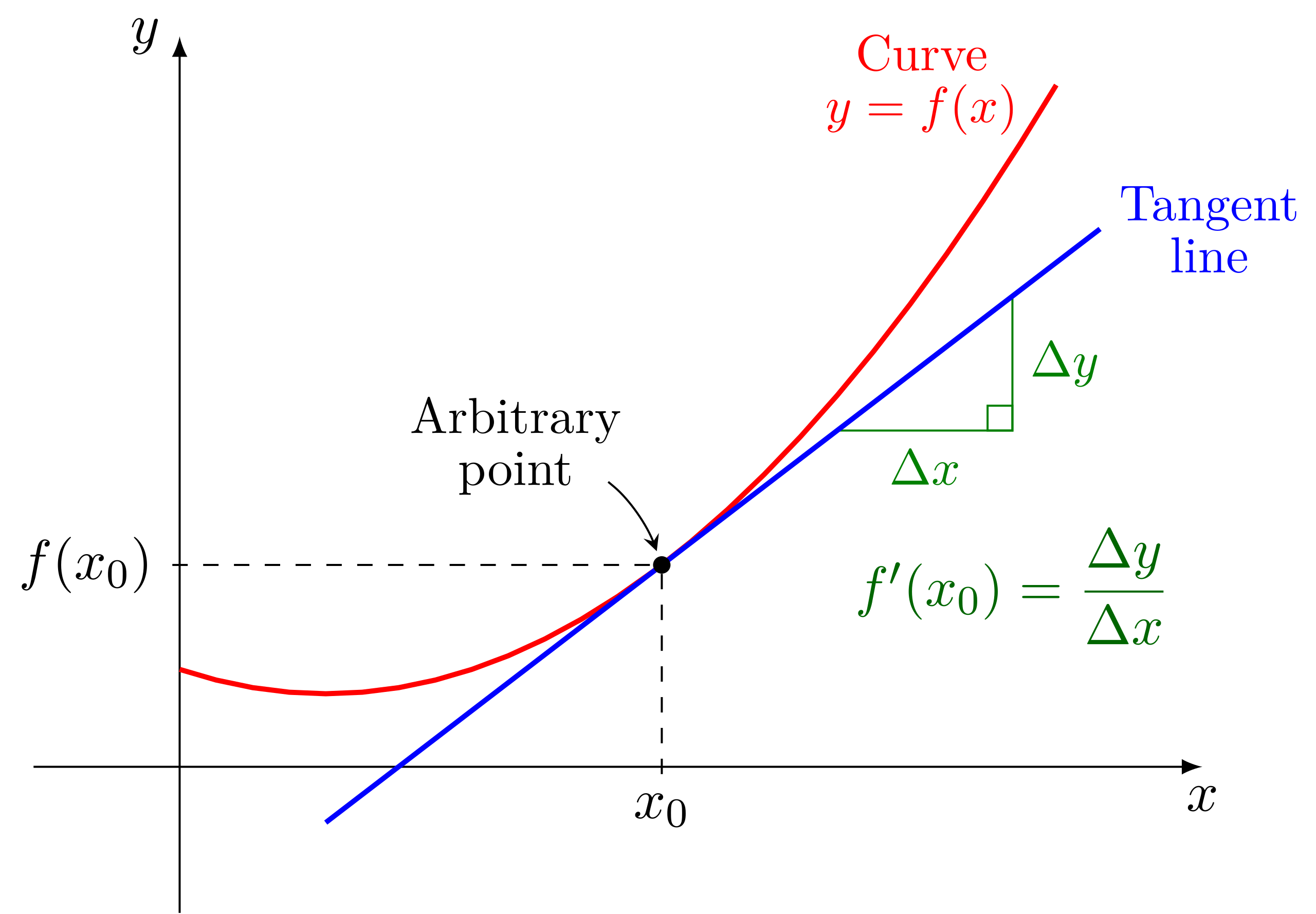
A curve is shown together with its tangent line at a single point, illustrating how the derivative at that point is represented by the slope of the tangent. The tangent line shares the same instantaneous direction as the curve at the point of contact. The axes allow visualization of how changes in $x$ relate to corresponding changes in $y$ along the tangent. Source.

Approaches to Estimating Derivatives Graphically

Drawing or Imagining a Tangent Line

To approximate the derivative at a point by visual inspection, students rely on constructing or imagining a tangent line that best fits the local behavior of the graph.

Key features to assess include:

• Direction: Whether the curve is increasing or decreasing at the point.

• Steepness: How rapidly the function rises or falls.

• Curvature: Whether the graph bends upward or downward, influencing tangent placement.

When a tangent line is drawn, the derivative at the point corresponds to its slope.

After identifying a reasonable tangent line, students use the graph’s scale markings to approximate this slope numerically, ensuring consistency with visible increments on the axes.

Inferring Tangent Slope from Nearby Secant Lines

In situations where a tangent is difficult to visualize, students may analyze slopes of secant lines drawn through the point of interest and nearby points.

Important ideas associated with this approach:

• The secant line’s slope approximates the average rate of change over an interval.

• As the second point moves closer to the target point, the secant slope better approximates the instantaneous rate of change.

• Converging secant slopes suggest the existence of a derivative at the point.

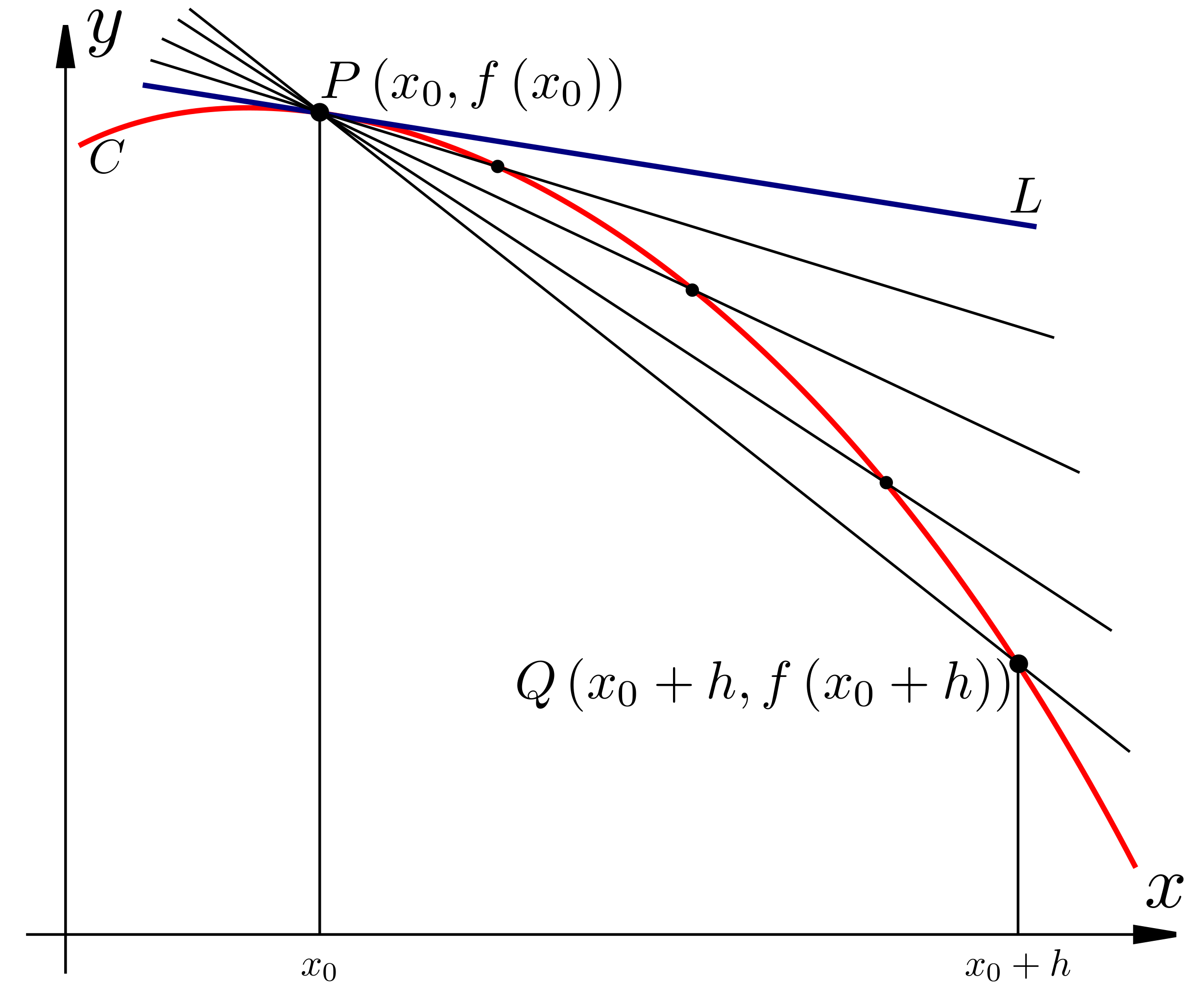
The graph shows a curve $C$, a tangent line $L$, and several secant lines connecting $x$ to $x+h$. As $h$ decreases, the secant slopes approach the slope of the tangent, illustrating how instantaneous rate of change emerges from average rates. Additional labels such as $x$, $x+h$, and $h$ provide visual clarity on the difference quotient $\frac{f(x+h)-f(x)}{h}$ even though this detail slightly exceeds the study notes’ minimal requirements. Source.

To use this strategy effectively, students select points close to the target point on both sides, ensuring the approximation captures the function’s local behavior.

Choosing a Method on a Given Graph

Students should evaluate which estimation approach is most appropriate for a particular graph by considering:

• Graph resolution: Whether the axes provide fine enough increments to measure slopes reliably.

• Smoothness of the function near the point: Smooth intervals favor tangent line estimation; irregular regions may require secant comparisons.

• Scale distortions: Unequal units on axes may mislead the eye, making careful reading essential.

Visual Cues for Interpreting Derivatives

Understanding how derivatives manifest graphically deepens intuition and strengthens estimation skills.

Key visual cues include:

• Positive derivative: Graph slopes upward from left to right.

• Negative derivative: Graph slopes downward from left to right.

• Zero derivative: Tangent line is horizontal, often corresponding to local maxima, minima, or saddle points.

• Large magnitude derivative: The graph is very steep; secant line approximations may require closer points for accuracy.

• Changes in concavity: Although concavity does not determine the derivative’s value, it influences how the tangent line hugs the curve.

Recognizing these cues helps students verify whether their estimated slope is reasonable.

Enhancing Accuracy in Graph-Based Estimation

To produce reliable derivative estimates from graphs, students should maintain a systematic strategy:

• Use multiple visual checks: compare tangent slope estimates with slopes of nearby secant lines.

• Consider symmetry: symmetric curves often yield predictable tangent behaviors at symmetric points.

• Stay within a small neighborhood: the smaller the interval, the closer the approximation reflects instantaneous change.

• Confirm consistency: re-evaluate estimates using alternative points or viewpoints on the same graph.

These techniques contribute to developing strong intuition as students build fluency in graphical differentiation.