This subsubtopic develops strategies for approximating a derivative at a point using numerical information, emphasizing how nearby function values reveal instantaneous change.

Estimating Derivatives from Tables of Values

Understanding the Goal of Numerical Estimation

When a function is presented only through a table of values, students must determine how the function changes near a specific input. Because a derivative represents an instantaneous rate of change, its value can be approximated by analyzing how function outputs vary over very small intervals around the target point.

Average Versus Instantaneous Change

The derivative at a point is built from the idea of average rate of change over intervals. As the interval around the point becomes smaller, the average rate approaches the instantaneous rate. Tables provide discrete data, so students use the smallest available intervals to estimate this limiting process.

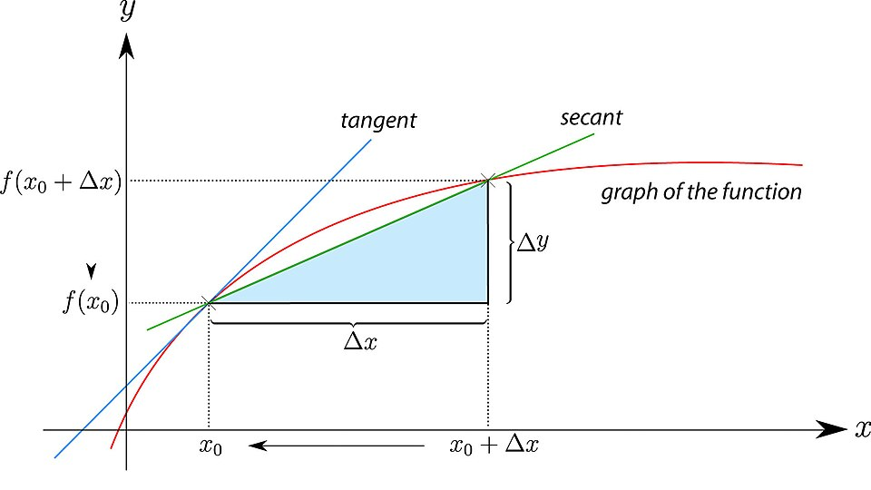
Differential quotient on a curve, with two nearby points connected by a secant line representing the average rate of change over a small interval. As the horizontal distance between the points shrinks, the secant slope approximates the derivative, reflecting the limit definition $f′(a) = \lim_{h \to 0} \dfrac{f(a+h) - f(a)}{h}$. The figure includes symbolic labels that slightly exceed syllabus requirements while remaining aligned with its concepts. Source.

Using One-Sided Difference Quotients

A one-sided difference quotient estimates the derivative using data entirely to the left or entirely to the right of the point of interest. These quotients are useful when only one direction of data is provided, such as at the edge of a table.

A sentence reminding students that difference quotients allow them to numerically approach the derivative ensures conceptual continuity with formal definitions.

Using Symmetric Difference Quotients

A symmetric difference quotient uses values on both sides of the point and typically provides a more accurate estimate of $f′(a)$ because it balances forward and backward changes.

Because symmetric quotients measure change centered at the point, they often better reflect the instantaneous rate, especially when the function behaves smoothly.

Interpreting Difference Quotients

A difference quotient, whether one-sided or symmetric, represents the instantaneous rate of change when interpreted as an estimate of the derivative. After computing the quotient, students must express its meaning in the context of the problem, particularly when tables describe real-world quantities.

To interpret an estimated derivative numerically, focus on:

• How quickly the output quantity is changing per unit of input.

• Whether the sign indicates increasing or decreasing behavior.

• The units associated with the change.

Choosing an Appropriate Quotient

The structure of the table determines which quotient is practical.

Consider the following guidelines:

• If data exists on both sides of the target value, prefer a symmetric difference quotient.

• If the data is missing on one side, use a one-sided difference quotient.

• If multiple possible intervals exist, choose the ones with the smallest $h$, reflecting values closest to the target.

These choices align the approximation as closely as possible with the conceptual limit that defines a derivative.

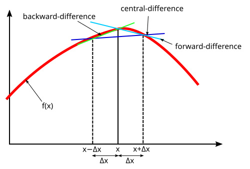
Diagram comparing forward, backward, and central finite differences, each representing a distinct numerical approach to estimating derivatives from nearby data. The central (symmetric) difference, which uses points on both sides of the target input, usually provides the most accurate approximation of $f′(a)$. The figure introduces brief notation that extends slightly beyond the syllabus but directly supports understanding of numerical derivative estimation. Source.

Accuracy and Limitations of Table-Based Estimates

Estimates from tables depend heavily on the spacing and quality of the data. Because table entries are finite and may not perfectly reflect the underlying function, the derivative estimate may include numerical error. Students should be aware of:

• Larger step sizes producing less accurate approximations.

• Irregular function behavior making symmetric and one-sided estimates differ more noticeably.

• Potential rounding errors if table values are approximated.

Despite these limitations, table-based methods remain powerful tools whenever symbolic or graphical information is unavailable.

The Derivative as a Limit Approached Numerically

Table-based estimation directly connects to the limit definition of the derivative. As the step size $h$ becomes smaller, the value of the difference quotient approaches the true derivative.

A table cannot make $h$ arbitrarily small, but it provides discrete values that approximate this limiting process. Students therefore treat the smallest available intervals as tangible representations of the limit concept.

Units and Contextual Interpretation

In applications, every derivative estimate must include appropriate units. For example, if $f(x)$ represents position in meters and $x$ represents time in seconds, then $f′(a)$ is given in meters per second. The numerical value alone is insufficient without its interpretation because the derivative communicates both magnitude and direction of instantaneous change.

Students must connect:

• The numerical result to the real-world behavior, such as speeding up, slowing down, or reversing.

• The sign of the estimate to whether the output is increasing or decreasing at that point.

Summary of Skills Needed for This Subsubtopic

Students should be able to:

• Recognize when to use one-sided or symmetric difference quotients.

• Approximate $f′(a)$ using the closest values in a table.

• Interpret numerical results as instantaneous rates of change.

• Understand how table-based estimates reflect the limit definition of the derivative.

• Communicate results clearly, including correct units and contextual meaning.