
AP Syllabus focus:
‘Use graphing technology or numerical derivative commands to approximate the value of a derivative at a point and compare with estimates from tables or graphs.’
Technology-based derivative approximations help students connect numerical, graphical, and symbolic reasoning by allowing rapid computation of slopes and instantaneous rates of change in diverse mathematical and real-world contexts.
Using Technology to Approximate Derivatives
Modern graphing tools and numerical commands provide efficient ways to approximate instantaneous rates of change, supporting conceptual understanding of how a derivative behaves locally. These tools typically estimate the slope of the tangent line by computing a numerical difference quotient, using values generated internally. Students should understand how these approximations relate to manual estimates from tables and graphs, while also recognizing the importance of correct syntax and interpretation when using technology.
Types of Technology Used in AP Calculus AB
Students may use graphing calculators, computer algebra systems, or digital graphing platforms. These tools usually include built-in numerical derivative functions that approximate at a chosen input value. Because technology relies on internal numerical methods, results may vary slightly depending on settings such as window scale or computation mode.
Graphing calculators often use commands like nDeriv, d/dx, or similar notation.
Graphing apps and software may use designated derivative tools or allow users to compute quotient-based approximations.
Handheld and online tools can display graphs, tables, and numeric output side by side to support interpretation.
Understanding Numerical Derivative Commands
When a calculator evaluates a derivative numerically, it approximates the derivative at a point by evaluating a difference quotient with a very small increment.
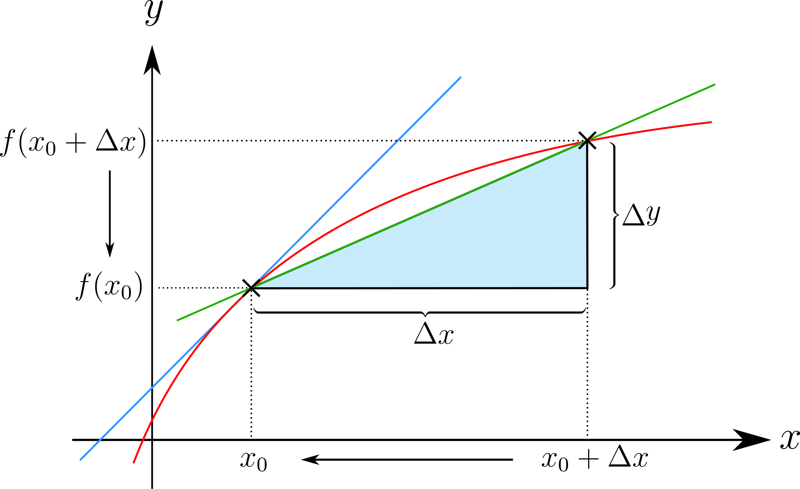
This diagram shows two points on a function connected by a secant line representing the difference quotient . The slope models the approximation used by numerical derivative commands. Additional labels identify points and segments without adding concepts beyond the AP Calculus AB syllabus. Source.
Numerical Derivative Command: A technology-based instruction that approximates the value of by computing a difference quotient with a very small step size determined internally by the device or software.
Numerical routines often employ a symmetric difference quotient for improved accuracy. Because these methods are approximations rather than symbolic computations, minor rounding differences are expected.
Approximating Derivatives Directly from Technology
Students can instruct a device to compute an approximate derivative at a point . The tool then outputs a number representing the tangent line’s slope at that location. This output corresponds to the instantaneous rate of change of the function, allowing analysis of how rapidly the function’s value changes relative to .
= A small positive increment selected by the algorithm
= Input value at which the derivative is approximated
After using such a command, students should interpret the resulting value within the context of the given problem. For example, a positive derivative indicates increasing behavior, while a negative value indicates decreasing behavior. Technology thus supports deeper reasoning about function behavior and modeling.
A single numerical value gains meaning only when related to the underlying function, its graph, or a real-world scenario. Therefore, interpreting the output is as important as obtaining it.
Comparing Technology-Based Results with Tables
Technology enables direct computation, whereas tables require estimation using nearby data. Students should be able to compare these approaches to strengthen conceptual understanding of how derivatives emerge from local linear behavior.
When working from a table, the student chooses entries near and forms a difference quotient. Technology, however, computes with values not limited to the table’s resolution, potentially increasing accuracy.
Key points for comparison include:
Whether a table’s spacing around is sufficiently small.
How symmetric and one-sided approximations differ.
The extent to which the technological estimate aligns with tabular behavior.
Situations where technology provides a clearer view of local trends than coarse data.
Comparing Technology-Based Results with Graphs
Graphical analysis offers a visual perspective on slope.
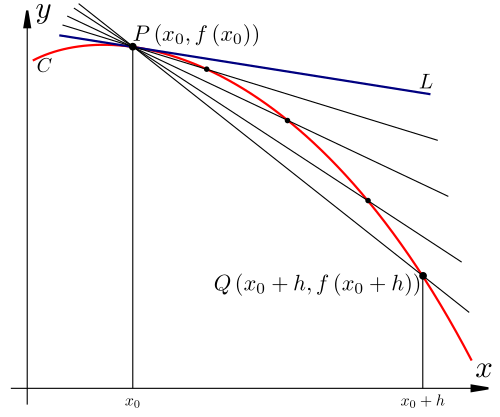
The diagram shows how secant lines between and approach the tangent line as becomes small. This visual reinforces the derivative as the limit of average rates of change. It mirrors how numerical tools approximate using very small intervals. Source.
Students may approximate the derivative by imagining or sketching a tangent line. Technology-based derivative tools complement this by supplying a numerical estimate that reinforces the graphical intuition.
Important considerations include:
Whether the tangent drawn visually appears to match the magnitude and sign of the technological estimate.
How steepness in the plotted graph correlates with the numerical derivative value.
The importance of selecting an appropriate window and scale, since distorted graphs can mislead interpretation.
Strengths and Limitations of Technology-Based Approximations
While technology improves efficiency and consistency, students should remain aware of its boundaries. Graphing windows may cause functions to appear flatter or steeper than they actually are. Likewise, numerical commands rely on step sizes that may not perfectly match the function’s behavior near sharp turns or points of rapid change.
Students should therefore:
Confirm that the graphing window is scaled reasonably.
Understand that numerical outputs are approximations, not exact values.
Cross-check results when graphs or tables suggest unusual behavior.
Use technology to support, not replace, conceptual reasoning about derivatives.
By using technology thoughtfully, students strengthen their understanding of instantaneous rates of change and develop confidence in interpreting derivatives across numerical, graphical, and contextual representations.
Practice Questions
A graphing calculator is used to approximate the derivative of a differentiable function f at x = 2. The calculator returns the value f'(2) = 3.7.
(a) State what this numerical output represents in terms of the behaviour of the function f.
(1 mark)
(1 mark total)
(a) 1 mark: States that the output 3.7 represents the instantaneous rate of change or slope of the tangent to the graph of f at x = 2, describing how quickly f is increasing at that point.
A function g is differentiable on an interval containing x = 4. A table of values for g near x = 4 is shown below:
x: 3.8, 3.9, 4.0, 4.1, 4.2
g(x): 5.6, 5.9, 6.3, 6.7, 7.0
A student uses technology to approximate g'(4) and obtains the value 3.2.
(a) Use the table to estimate g'(4) using a symmetric difference quotient.
(b) Compare your estimate with the technology-generated value and comment on why they might differ.
(c) Explain how decreasing the table spacing (for example, using values closer to x = 4) would be expected to affect the accuracy of the manual estimate.
(4 marks)
(4 marks total)
(a) 2 marks:
1 mark for correctly forming the symmetric difference quotient using values at x = 3.9 and x = 4.1.
Calculation: (6.7 − 5.9) divided by (4.1 − 3.9).1 mark for the correct numerical estimate (4.0).
(b) 1 mark:
A valid comparison mentioning that 4.0 differs from 3.2, with an explanation such as technology using a much smaller interval, more precise internal values, or reduced rounding error.
(c) 1 mark:
Correct statement that using values closer to x = 4 would generally improve accuracy because the symmetric difference quotient would better approximate the instantaneous rate of change.
FAQ
Most graphing calculators use an internally fixed but very small step size that balances precision with the limits of floating-point arithmetic. The exact value is usually not shown to the user.
A step size that is too small can cause rounding errors, while one that is too large reduces accuracy, so calculators use a default setting optimised for typical school-level functions.
Different devices use different algorithms, such as symmetric or one-sided difference quotients, and may choose different internal step sizes.
Small differences in graphing resolution, rounding settings, or stored precision can also produce variations in computed slopes.
Numerical approximations are less stable when the function changes rapidly over small intervals or when the function has sharp curvature.
Values may also drift if the function is extremely large or small near the evaluation point, increasing rounding effects.
A poorly chosen window might distort the apparent steepness of a curve, making it harder to judge whether the numerical derivative seems reasonable.
A suitable window allows the user to visualise local behaviour clearly, compare the steepness with the computed value, and spot anomalies such as vertical exaggeration.
It is wise to be cautious when the output contradicts nearby function behaviour visible on the graph or suggested by a table of values.
Potential warning signs include abrupt jumps in output, instability when the evaluation point is changed slightly, or contexts where the function is known to behave erratically near the chosen input.
