AP Syllabus focus:
‘Using a slope field, students reason about families of solution functions, including their qualitative behavior, possible equilibrium solutions, and how solutions change as the independent variable increases.’
Understanding Long-Term Behavior in Slope Fields
Slope fields allow students to visualize how differential equation solutions behave as the independent variable grows large, revealing long-term tendencies that cannot always be seen algebraically within introductory contexts. These visual cues help link differential equations to qualitative solution behavior.
Families of Solutions in a Slope Field
A family of solutions refers to the complete set of curves that satisfy a given first-order differential equation. In a slope field, this family appears as many possible solution paths threading through the grid of slope segments. Each path reflects how a different initial condition produces a distinct member of the family.

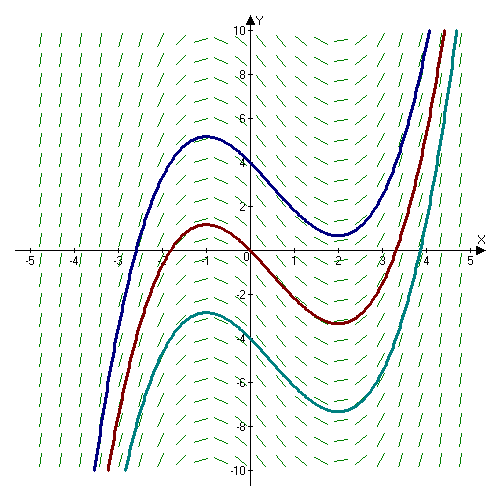
This diagram shows a slope field for a first-order differential equation with several solution curves superimposed. Each colored curve represents a particular solution determined by a different initial condition, while the short dashed segments indicate the local slopes given by the differential equation. The extra detail that the underlying equation is is not required by the syllabus, but it does not change the qualitative interpretation of the solution family. Source.
Family of Solutions: A collection of all solution curves to a differential equation, each determined by a particular initial condition and together representing every possible behavior permitted by the equation.
Because slope fields emphasize qualitative understanding rather than explicit formulas, they help students identify how solution curves evolve, diverge, or stabilize as the independent variable increases.
Qualitative Behavior and Long-Term Trends
Qualitative behavior describes how solution curves behave without requiring formulaic solutions. When analyzing slope fields for long-term behavior, students look for overall patterns rather than point-by-point computations. Key features include how the slopes change across the grid and whether curves approach, avoid, or diverge from important structures in the field.
Indicators of Long-Term Behavior
Students should look for visual cues such as:
Convergence, where multiple solution curves tend toward the same long-term value or shape.
Divergence, where nearby solution curves spread apart as the independent variable increases.
Leveling off, where slopes become nearly zero and solution curves flatten.
Directional consistency, where curves move in a predictable pattern indicating sustained growth or decay.
These indicators reveal whether a solution will increase without bound, decrease, or settle near a constant value over time.
Equilibrium Solutions in Long-Term Behavior
Many differential equations possess equilibrium solutions, which play a central role in determining long-term behavior.
Equilibrium Solution: A constant solution to a differential equation for which the derivative equals zero, meaning the dependent variable does not change over time.
A sentence describing why this matters: Equilibrium solutions visually appear as horizontal lines in the slope field where the slope segments have zero inclination.
Stability of Equilibria
Slope fields can suggest whether an equilibrium is stable or unstable, based solely on the surrounding slopes.
A stable equilibrium attracts nearby solution curves as the independent variable increases.
An unstable equilibrium repels nearby solution curves, causing them to diverge away.
A semi-stable equilibrium attracts from one side and repels from the other.
These observations provide insight into the future behavior of solutions.

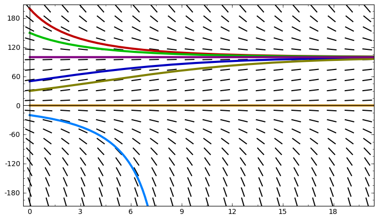
This figure presents a slope field for a logistic differential equation together with several solution curves. The horizontal lines at the equilibrium values show where the derivative is zero, and the colored solution curves demonstrate how different initial values either converge toward or diverge from these equilibria as time increases. The specific functional form and the numerical values used are extra detail beyond the syllabus, but the qualitative behavior is exactly the kind students interpret in AP Calculus AB. Source.
How Solutions Change as the Independent Variable Increases
Interpretation of long-term behavior relies on recognizing how solution curves adapt to the slope structure further to the right in the field.
Recognizing Growth, Decay, or Flattening
As increases, solution curves follow the directional cues given by the slope segments:
Sustained positive slope suggests long-term growth.
Sustained negative slope indicates long-term decay.
Slope approaching zero points to leveling behavior, hinting that the solution may approach an equilibrium.
When slopes alternate between positive and negative regions, students note cyclical or oscillatory patterns, although AP Calculus AB typically emphasizes non-oscillatory first-order behavior.
A normal explanatory sentence ensures spacing before any equation, though none is required next.
Using Slope Fields to Compare Different Long-Term Behaviors
Different initial conditions may lead to dramatically different long-term outcomes even within the same slope field. Students use the grid of slopes to track these distinctions, observing how initial placement influences the entire future trajectory.
Distinguishing Between Solution Paths
By following visual slope cues:
Two curves starting near each other may diverge widely, indicating sensitivity to initial conditions.
Curves starting on opposite sides of an equilibrium may move toward different limiting values.
Some curves may approach a finite constant, while others may increase or decrease without bound.
Recognizing these patterns helps students interpret the overall structure of the differential equation’s behavior.
Visual Reasoning and Interpretation Skills
Interpreting long-term behavior is ultimately a matter of reasoning with the slope field’s visual information:
Key Skills to Develop
Identifying where slopes are zero, positive, or negative.
Tracking how slope magnitude changes over the grid.
Understanding the interaction between initial conditions and slope direction.
Recognizing whether solution curves converge, diverge, or remain separated.
Describing limiting behavior as the independent variable becomes large.
These skills align directly with the syllabus expectation that students use slope fields to reason about families of solutions, equilibrium behavior, and how solutions change as the independent variable increases.
FAQ
Look at the magnitude of the slope segments near the equilibrium. Larger slopes indicate faster movement towards (or away from) the equilibrium, while very small slopes suggest slow convergence.
You can also compare how spaced the solution curves would be if sketched: tightly packed curves usually indicate rapid settling, whereas gradual flattening shows slower approach.
A slope field often contains different regions where the slopes change sign or magnitude. These regions can guide solutions in different directions.
When an initial value places a solution in a region dominated by positive slopes, it will rise long-term, whereas an initial value in a region dominated by negative slopes will fall. This creates long-term behaviour that depends strongly on where the solution begins.
Yes. Look for slope segments that remain consistently positive (or increasingly positive) as x increases, causing curves to rise without flattening.
If solution curves would need to leave the visible grid to continue following the slope trends, this suggests unbounded growth. Sparse or steep segments toward the right side of the field often signal this behaviour.
Multiple horizontal bands of zero slope indicate multiple equilibrium levels. These appear as rows of flat slope segments where the directional tendency changes above or below each line.
In some cases, you may see alternating behaviour such as one equilibrium attracting curves and another repelling them, depending on the orientation of surrounding slopes.
Check whether the slopes immediately above and below the equilibrium have similar steepness and pattern. If the slope magnitudes mirror each other, the behaviour may be roughly symmetric.
However, if the slope segments above the equilibrium are much steeper or change more rapidly than those below, the long-term approach or divergence will differ noticeably across the two sides.
Practice Questions
Question 1 (1-3 Marks)
A slope field for the differential equation dy/dx = f(x, y) is shown. Several solution curves appear to level off as x increases.
(a) State what this suggests about the long-term behaviour of these solutions.
(b) Identify the type of solution that the curves appear to be approaching.
Question 1
(a) 1 mark: States that the solutions approach a constant value or level off.
(b) 1 mark: Identifies the limiting value as an equilibrium solution.
Total: 2 marks
Question 1 (4-6 Marks)
Consider the slope field for a differential equation dy/dx = g(x, y). The field shows that all solution curves above y = 3 decrease towards y = 3 as x increases, while all curves below y = 3 increase towards y = 3.
(a) Explain why y = 3 is an equilibrium solution.
(b) State whether this equilibrium is stable or unstable, giving a reason.
(c) A solution curve begins at the point (0, 5). Describe fully the long-term behaviour of this solution as x increases.
(d) A different solution curve begins at the point (0, −1). Describe fully how its long-term behaviour compares with the curve beginning at (0, 5).
Question 1
(a) 1 mark: States that y = 3 is an equilibrium because dy/dx is zero there or the slope segments are horizontal.
(b) 1 mark: Identifies the equilibrium as stable.
(c) 1 mark: States that the solution starting at (0, 5) decreases towards y = 3 as x increases.
(d) 1 mark: States that the solution starting at (0, −1) increases towards y = 3 as x increases.
(e) 1 mark: Clearly compares the two solutions, stating that both approach the same stable equilibrium from opposite sides.
Total: 5 marks

