
AP Syllabus focus:
‘Introduction to the key characteristics of quantitative data distributions: shape, center, variability (spread), and unusual features.
- Describing shape: Understanding the significance of symmetry, skewness (right or left), unimodality, bimodality, and uniformity.
- Identifying center: Exploring measures that indicate the central tendency of the data.
- Assessing variability: Discussing the range, interquartile range (IQR), and standard deviation as measures of spread.
- Highlighting unusual features: Recognizing outliers, gaps, clusters, and multiple peaks within distributions.
- Skill 2.A: Enhancing the ability to thoroughly describe quantitative data distributions, including all mentioned aspects.’
Understanding the characteristics of a quantitative distribution is essential for identifying meaningful patterns, describing data behavior, and interpreting results with clarity and context in statistical analysis.
The Fundamental Components of a Distribution
A distribution conveys how values in a quantitative dataset are arranged. AP Statistics emphasizes four core characteristics: shape, center, variability, and unusual features. Together, these features provide a comprehensive description of how data values are positioned and how they behave relative to one another.
Shape of a Distribution
Shape refers to the overall visual form or pattern displayed when quantitative data are graphed. Recognizing shape helps reveal underlying tendencies and behaviors of the dataset.
Symmetry and Skewness
A distribution is symmetric when its left and right sides are mirror images. When symmetry occurs, measures of center often align closely, reflecting balanced data.
Symmetry: A property of a distribution in which the left and right sides are approximately identical in shape and frequency.
A distribution is skewed if one tail is longer than the other. Right (positive) skew has a longer tail on the right side, while left (negative) skew has a longer tail on the left. Skewness is important because it influences which measure of center best reflects the distribution’s behavior.
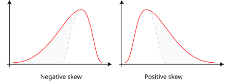
The diagram compares negatively and positively skewed distributions, illustrating how the direction of the tail affects the overall shape and interpretation of the data. Source.
Modality
Modality describes the number of significant peaks in a distribution.
Mode: A value or region of values where the distribution reaches a local maximum in frequency.
A unimodal distribution has one main peak. Bimodal distributions have two prominent peaks, often indicating two distinct subgroups within the data. A uniform distribution displays roughly equal frequencies across values, indicating no dominant peak.
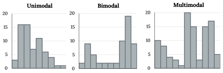
These histograms compare one-peak, two-peak, and three-peak distributions, clarifying how modality is determined and how multiple peaks reveal structural patterns in data. Source.
Between these ideas, understanding shape is critical because it directly influences interpretation, comparisons, and the choice of numerical summaries appropriate for the data.
Measures of Center
The center of a distribution identifies a typical or representative value for the dataset. AP Standards highlight that identifying center is essential for capturing the “middle” of the data’s numerical behavior.
Common Measures
The most frequently used measures of center are the mean and the median.
Median: The middle value in an ordered dataset, with half of the observations above and half below.
The center is important because it offers a reference point that helps describe the distribution relative to its shape and spread.
Measures of Variability
Variability (spread) indicates how dispersed the data values are. AP Statistics requires familiarity with range, interquartile range (IQR), and standard deviation when describing distributions.
Range and IQR
The range captures the distance between the maximum and minimum values, offering a quick sense of overall spread. The IQR, which spans the middle 50% of data, provides a more resistant measure of spread.
EQUATION
= First quartile (25th percentile)
= Third quartile (75th percentile)
The IQR is especially useful when distributions are skewed or contain outliers because it focuses only on the central portion of the data.
Standard Deviation
Standard deviation measures the typical distance of data points from the mean, allowing students to quantify how tightly or loosely data cluster around the center.
EQUATION
= Sample standard deviation
= Individual data value
= Sample mean
= Number of data points
Standard deviation is particularly informative when the distribution is reasonably symmetric.
A deep understanding of variability complements the center because together they provide a fuller picture of how data behave.
Unusual Features in Distributions
Identifying unusual features is a key expectation of this subsubtopic. These features highlight irregular or noteworthy characteristics that may require further investigation.
Outliers, Gaps, and Clusters
Outliers are data values that differ markedly from the overall pattern. Their presence can affect the mean, standard deviation, and perceived shape of the distribution.
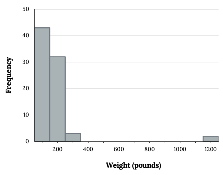
The histogram highlights how an outlier appears as a data point far from the main cluster, influencing center and spread and signaling potential special conditions in the dataset. Source.
Outlier: An observation that falls unusually far from the overall pattern of the data.
A distribution may also exhibit gaps, which are regions where no observations occur. In contrast, clusters represent areas where many observations are concentrated. Multiple peaks or separated clusters often suggest the influence of different processes, subpopulations, or conditions within the dataset.
Recognizing such unusual features supports meaningful interpretation and helps justify conclusions in context, which is essential for meeting AP skill expectations.
FAQ
Small samples often produce irregular or misleading shapes because each observation carries more weight. A distribution may seem skewed, multimodal, or contain gaps simply due to the limited number of data points.
Larger samples tend to smooth out random fluctuations, making features such as symmetry, skewness, and modality more reliable indicators of the true underlying population distribution.
A distribution is truly multimodal when multiple peaks correspond to genuine subgroups or underlying processes.
Random peaks may occur when:
• the sample size is small
• the bin width in a histogram is inappropriate
• the distribution is heavily influenced by random variation
To distinguish them, consider context, increase the sample size if possible, or examine alternative graphical displays.
Certain processes generate values that fluctuate around a central point, producing an approximately symmetric pattern despite asymmetry in the mechanism.
Symmetry can also emerge when different sources of variation combine. For example, multiple small influences acting together often produce a roughly symmetric, mound-shaped distribution.
Clusters may form when individuals behave differently under varying conditions, even within the same group.
Possible reasons include:
• Changes across time (morning vs afternoon behaviour)
• Environmental or situational effects
• Hidden variables influencing subsets of observations
Clusters often highlight structure in the data that requires contextual interpretation.
Outliers can be difficult to classify because unusual values may represent genuine variation rather than errors.
Challenges include:
• natural extremes in heavy-tailed distributions
• measurement inconsistencies
• context-specific thresholds for what counts as unusual
Outlier detection is most reliable when combined with contextual knowledge, not solely graphical or numerical rules.
Practice Questions
Question 1 (1–3 marks)
A histogram displays the distribution of the number of minutes students spend on homework each night. The histogram shows a long tail to the right.
(a) State the shape of this distribution.
(b) Identify the measure of centre that would be most appropriate to report and explain why.
Question 1 (1–3 marks)
(a) 1 mark:
• States that the distribution is right-skewed / positively skewed.
(b) 1–2 marks:
• 1 mark for identifying the median as the appropriate measure of centre.
• 1 mark for explaining that the median is resistant to extreme values or skewness, whereas the mean is pulled in the direction of the skew.
Question 2 (4–6 marks)
A researcher records the daily number of customers entering a small café over a 30-day period. The dotplot of the data shows two clear clusters of values: one cluster centred around 25 customers per day and another cluster centred around 60 customers per day. A single unusually high value of 120 customers also appears.
(a) Describe fully the key characteristics of this distribution, referring to shape, centre, variability, and unusual features.
(b) Suggest a plausible explanation for the presence of clusters in this context.
(c) Comment on how the outlier might affect the choice of summary statistics.
Question 2 (4–6 marks)
(a) Up to 3 marks:
• 1 mark for describing the shape as bimodal.
• 1 mark for identifying two centres corresponding to the two clusters (around 25 and 60).
• 1 mark for referring to variability (e.g., spread between clusters or general dispersion).
• 1 mark for identifying the outlier at 120 as an unusual feature.
(Maximum 3 marks for part (a).)
(b) 1 mark:
• Provides a plausible explanation for the clusters, such as weekdays vs weekends, differing customer patterns, or special events.
(c) Up to 2 marks:
• 1 mark for stating that the outlier would influence non-resistant statistics such as the mean and standard deviation.
• 1 mark for stating that resistant statistics such as the median and IQR would be more appropriate due to the extreme value.
