
AP Syllabus focus:
‘Introduction to the five-number summary as a key concept in descriptive statistics, consisting of the minimum, first quartile (Q1), median, third quartile (Q3), and maximum data values.
- Explaining the significance of each component in providing a compact summary of the distribution's range and central tendency.
- Skill 2.B: Developing the ability to compute and understand the five-number summary for a set of quantitative data.’
The five-number summary provides a compact, powerful way to describe the distribution of a quantitative variable, capturing its center, spread, and extreme values. It forms the foundation for several graphical and numerical tools in statistics, especially boxplots, and helps highlight important distributional features efficiently and clearly.
The Role of the Five-Number Summary
A five-number summary condenses an entire dataset into five key descriptive statistics. These values are intentionally chosen because they mark essential boundaries of the distribution. Together, they offer a structured overview of how the data are spread, where the middle lies, and whether extreme observations influence interpretation. The summary is especially useful when the dataset is large or when the distribution is skewed, irregular, or contains outliers.
Components of the Five-Number Summary
The five components appear in a specific order from smallest to largest. Each value describes an essential point in the data's distribution.
Minimum
First Quartile (Q1)
Median
Third Quartile (Q3)
Maximum
Each term has a precise meaning grounded in descriptive statistics.
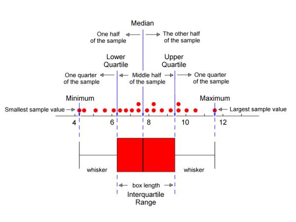
This labeled boxplot illustrates the five-number summary on a number line, identifying the minimum, Q1, median, Q3, and maximum. The diagram also shows how the middle half of the sample forms the interquartile range and how the data divide into quarters. The additional annotations extend slightly beyond the syllabus but support a deeper understanding of quartiles. Source.
Minimum
The minimum is the smallest observed value in the dataset. It marks the lower boundary of the distribution and serves as the starting point for interpreting variability. Because it is sensitive to unusually low values, it provides insight into potential lower-end outliers.
First Quartile (Q1)
First Quartile (Q1): The value that separates the lowest 25% of the data from the remaining 75% when the dataset is ordered.
Q1 helps identify the lower segment of the distribution and is a key element for assessing spread within the lower half of the data. It is resistant to extreme values and provides a stable indicator for describing distribution shape.
Median
Median: The middle value of an ordered dataset, with 50% of observations below it and 50% above it.
As a measure of center, the median is crucial for understanding the distribution’s balance point. Unlike the mean, it is not affected by outliers, making it especially effective in skewed distributions.
Third Quartile (Q3)
Third Quartile (Q3): The value that separates the lowest 75% of the ordered data from the highest 25%.
Q3 provides a view into the upper portion of the distribution. Like Q1, it is resistant to outliers and assists in evaluating how the data behave toward the higher end.
Maximum
The maximum is the largest observed value in the dataset. It sets the upper boundary of the data and can reveal unusually high observations that warrant attention. Differences between the maximum and other summary values contribute to interpretations of skewness and spread.
How the Five-Number Summary Describes a Distribution
The five-number summary creates a structured framework that captures several essential aspects of a dataset.
Understanding Spread
The summary establishes the data’s overall range, defined as the distance between the minimum and maximum. The distance between Q1 and Q3—known as the interquartile range (IQR)—highlights the spread of the central portion of the distribution. These measures help students understand whether the data are tightly clustered or widely dispersed.
EQUATION
= First quartile (lower 25%)
= Third quartile (upper 25%)
Between these values, one can evaluate how consistent the central data are before encountering extreme values.
Understanding Center
The median serves as the central anchor for the five-number summary. When Q1 and Q3 are equidistant from the median or close to equidistant, the distribution may appear relatively symmetric. Uneven spacing can hint at skewness even before a graph is drawn.
Detecting Potential Outliers and Unusual Features
Because the summary identifies the extreme values and the central range, it helps reveal when observations at the minimum or maximum appear unusually far from the rest of the distribution. Students often use the values of Q1 and Q3, combined with the IQR, to support later formal outlier detection techniques.
Supporting Visualization and Interpretation
The five-number summary is the foundation of boxplots, graphical tools that display data distribution using these five key values.
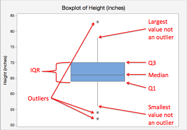
This boxplot diagram shows how the minimum, first quartile (Q1), median, third quartile (Q3), and maximum (here, the smallest and largest non-outlier values) appear graphically. The box visualizes the middle 50% of data between Q1 and Q3, with the median marked inside. The outlier symbols and “not an outlier” labels add minor additional context beyond the syllabus. Source.
Understanding each component of the summary directly improves a student’s ability to interpret boxplots, compare groups visually, and justify claims based on distribution shape, spread, and location.
Why the Five-Number Summary Matters
The summary provides a sturdy, context-independent method for describing a dataset without computational complexity. It is especially effective for highlighting variations, identifying potential data issues, and forming an initial interpretation of the distribution before applying more advanced techniques.
FAQ
Adding new extreme values typically changes only the minimum or maximum, leaving Q1, the median, and Q3 unchanged unless the new values alter the ordering around those quartiles.
This means the range increases immediately, but the interquartile range remains stable unless many new values cluster near the quartile boundaries.
The minimum and maximum are non-resistant and change dramatically with outliers.
However, Q1, the median, and Q3 are resistant because they depend only on the relative ordering of data, not the magnitude of extreme observations.
This combination makes the five-number summary a partly resistant tool that still captures unusual extremes.
Quartiles divide data into equal counts, not equal widths on the number line.
If the numeric distance between Q1 and the median is much smaller than between the median and Q3, it suggests clustering in one region and wider spread in another.
This uneven spacing can point to subtle skewness or the presence of gaps within particular segments of the distribution.
Yes. Distinct data sets can produce identical five-number summaries even if their internal structures differ.
For example, one may contain clusters while another is uniformly spread between quartile boundaries.
Because the summary compresses data into only five values, it is not unique to a single distribution.
It can be limiting when the data display complex internal patterns, such as multiple clusters or cyclical structures, because these details are hidden within quartile boundaries.
It is also insufficient when the exact values of observations matter, such as in contexts requiring precise measurement or sensitivity to individual deviations.
In such cases, pairing the summary with graphical tools or full data inspection is recommended.
Practice Questions
Question 1 (1–3 marks)
A data set consists of the following five-number summary:
Minimum = 12, Q1 = 18, Median = 24, Q3 = 31, Maximum = 47.
State two features of the distribution that can be identified directly from this five-number summary.
Question 1 (2 marks)
Award 1 mark for each correct feature, up to 2 marks.
Accept any two of the following:
The range of the data can be seen (maximum minus minimum).
The median identifies the centre of the distribution.
The interquartile range can be determined (Q3 minus Q1).
The positions of the quartiles indicate how the data are spread across the distribution.
The presence of large gaps between quartiles may suggest skewness or uneven spread.
Question 2 (4–6 marks)
A researcher records the completion times (in minutes) of participants solving a puzzle. She calculates the following five-number summary:
Minimum = 9, Q1 = 14, Median = 19, Q3 = 28, Maximum = 55.
(a) Comment on the spread of the central 50% of the data.
(b) Explain how the five-number summary suggests the presence of potential outliers.
(c) Describe what the summary indicates about the skewness of the distribution, giving a justification.
Question 2 (5 marks)
(a) Comment on the spread of the central 50% (1 mark)
1 mark: Correctly states that the IQR is 14 minutes (28 − 14) or states that the central 50% of the data is moderately spread.
(b) Explanation of potential outliers (2 marks)
1 mark: Identifies that the maximum value (55) is far from Q3.
1 mark: States that such a large distance suggests possible high-value outliers or unusually large observations.
(c) Description of skewness with justification (2 marks)
1 mark: States that the distribution is likely right-skewed (positively skewed).
1 mark: Justifies by noting that the upper half (median to maximum) is more widely spread than the lower half (minimum to median), or that the maximum is much further above Q3 than the minimum is below Q1.
