
AP Syllabus focus:
‘VAR-5.A.3: Detail how a probability distribution for a discrete random variable can be represented using graphs, tables, or functions, showing the probabilities associated with each value of the random variable. VAR-5.A.4: Also introduce the concept of a cumulative probability distribution and how it can be represented to show probabilities up to each value of the random variable.’
In this section, you will learn how discrete random variables use probability distributions, graphs, tables, and functions to describe long-run behavior of random processes mathematically.
Representing probability distributions for discrete random variables
A probability distribution for a discrete random variable organizes all possible numerical values the variable can take and the probability attached to each of those values. For AP Statistics, you must be able to read, interpret, and compare distributions given in tables, functions, and graphs, and you must also understand what a cumulative probability distribution shows about “up to” or “at most” probabilities.
Discrete random variable: A numerical variable whose possible values form a countable set (such as whole numbers), each with an associated probability.
A discrete random variable typically arises from counting something, such as the number of successes in a fixed number of trials, and its probability distribution captures the long-run relative frequency pattern of those counts.
Probability distribution (discrete): A description that lists every possible value of a discrete random variable together with the probability of each value, with all probabilities between 0 and 1 and summing to 1.
Because the distribution must assign probabilities that sum to 1, it acts as a complete model for how chance determines the variable’s behavior.
Tabular representations of probability distributions
One of the most direct ways to represent a discrete probability distribution is with a table. A probability table typically contains:
• A row or column listing each possible value of the random variable.
• A corresponding row or column listing the probability of each value.
This representation emphasizes that:
• Every possible outcome value appears exactly once in the table.
• Each listed probability is between 0 and 1.
• The probabilities for all listed values add up to exactly 1.
A table makes it easy to locate the probability of a specific value and to combine probabilities for sets of values (events) by adding the relevant entries.
Functional representations: probability mass functions
A probability distribution for a discrete random variable can also be expressed as a function, often called a probability mass function (pmf). Instead of listing values in a table, the function assigns a probability to each possible value using algebraic notation.
EQUATION
= Probability that the random variable X takes the value x
= Discrete random variable defined on a countable set of possible values
The function representation highlights two key properties:
• For every allowed value x, p(x) is between 0 and 1.
• The sum of p(x) over all possible values of x is equal to 1.
Using a function is especially helpful when the distribution follows a clear rule, since it allows you to compute probabilities for many values without writing out a long table.
Graphical representations: bar graphs and probability histograms
Probability distributions for discrete random variables are often visualized using bar graphs or probability histograms.
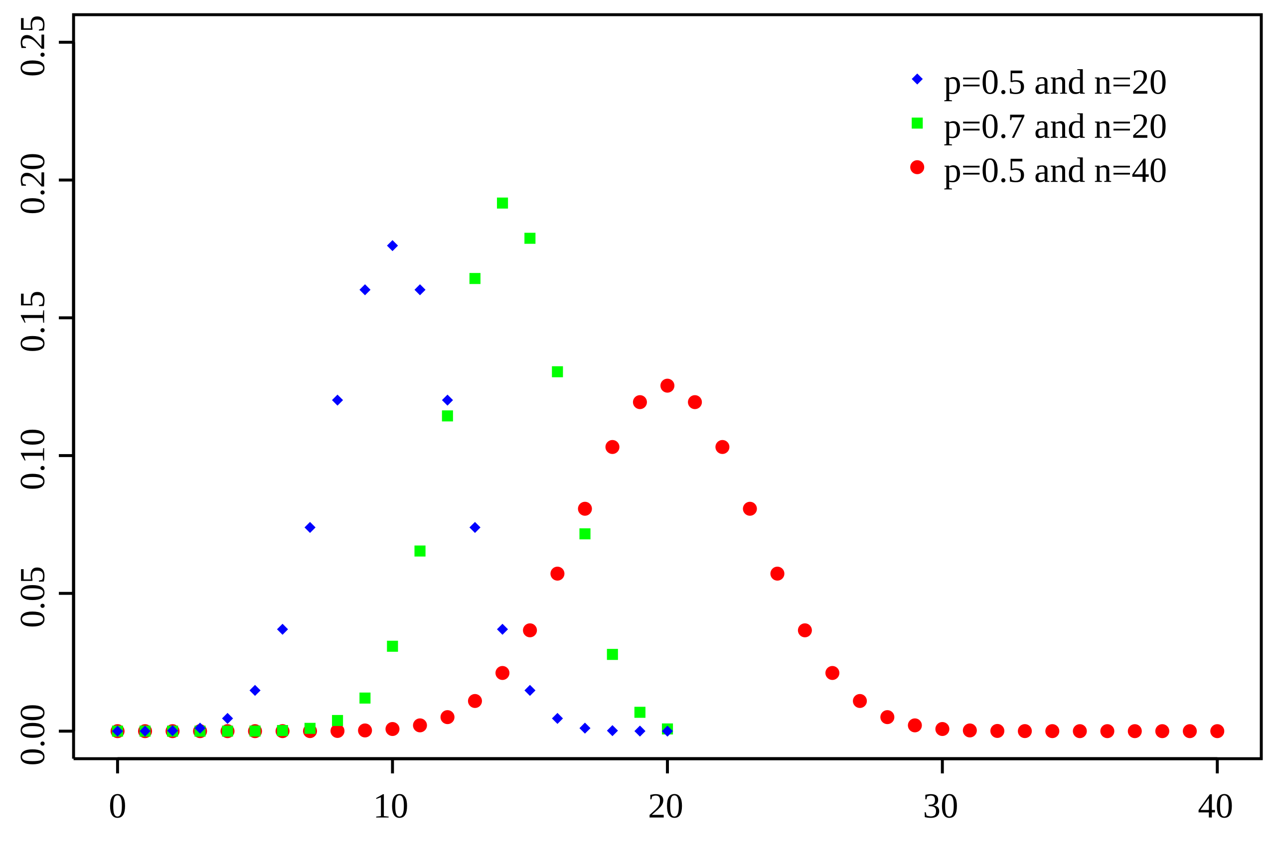
This graph shows binomial probability mass functions, with each dot representing the probability of a specific discrete outcome. Although points are used instead of bars, the image illustrates how each value of a discrete random variable has its own probability. Multiple curves for different parameter values are included as extra detail beyond the syllabus requirements. Source.
In these graphs:
• The horizontal axis shows the possible values of the random variable.
• The vertical axis shows the probability assigned to each value.
• Each value has a separate bar whose height corresponds to its probability.
Graphical representations help you quickly assess features of the distribution such as:
• Where the distribution is concentrated (values with relatively high probability).
• Whether the distribution is symmetric, skewed, or has gaps in possible values.
• How spread out the likely values of the random variable are.
Even though the bars may resemble a histogram for quantitative data, here each bar’s height is a probability, not a frequency count.
Cumulative probability distributions
Beyond showing the probability of each individual value, it is often useful to know the probability that the random variable is less than or equal to a given value. This is the role of the cumulative probability distribution, sometimes called the cumulative distribution function (cdf).
Cumulative probability distribution: A representation that gives, for each possible value x of a discrete random variable, the probability that the variable is less than or equal to x.
Cumulative distributions answer questions involving “up to,” “at most,” or “no more than” by gradually accumulating probabilities from the smallest value upward.
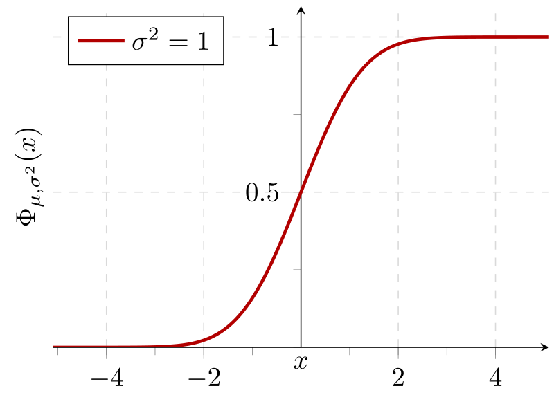
This image shows a cumulative distribution function, where the height of the curve represents the probability that the random variable takes a value less than or equal to x. As x increases, cumulative probability rises from 0 toward 1. The use of a continuous normal distribution includes extra detail beyond the syllabus but clearly illustrates the idea of accumulating probability. Source.
EQUATION
= Cumulative probability that X is less than or equal to the value x_k
= Individual possible values of the discrete random variable X
Cumulative probability distributions can be represented in several ways:
• Tables, where each row includes a value x and the cumulative probability up to that value.
• Graphs, where the horizontal axis lists values of the variable and the vertical axis shows F(x), typically forming a step-shaped function that increases as x increases.
Using cumulative distributions in practice
Cumulative distributions allow you to:
• Determine how likely it is that the random variable falls within a given range that starts at the smallest value.
• Compare how quickly probability accumulates for different random variables, revealing differences in center and spread.
• Interpret probabilities in context by translating statements like “the probability of at most k” into cumulative probabilities read from a table or graph.
Together, representations by tables, functions, graphs, and cumulative distributions provide complementary views of the same underlying discrete probability model, giving you flexible tools for analyzing random behavior in AP Statistics.
FAQ
Tables are best when you need to read exact probabilities for each value quickly, especially when precision is essential.
Graphs are more helpful when the goal is to compare shapes, judge symmetry, or visually assess concentration of probability.
Use a table for accuracy and a graph for pattern recognition; both represent the same information but emphasise different aspects of the distribution.
A discrete cumulative distribution only increases at values the random variable can actually take, so the graph must move in jumps rather than continuously.
Each step corresponds to adding the probability of a specific value, which creates a staircase-like shape.
A smooth curve would imply a continuous set of possible values, which does not apply to discrete random variables.
Graphs allow quick visual comparison of:
• Skewness or symmetry
• Concentration around certain values
• The presence of gaps or unusually high/low probabilities
These features may be hidden in a table, where equal formatting makes it harder to judge magnitude or structure at a glance.
This can occur when the variables assign probability to different individual values but accumulate to the same totals by key points.
For example, one variable may spread probability across values differently, yet both still reach the same probabilities at or below chosen cut-offs.
Cumulative distributions highlight overall accumulation, not the distribution’s exact internal allocation.
Typical errors include:
• Treating the graph like a histogram of frequencies rather than probabilities
• Assuming the bars must touch, which is not required for discrete variables
• Misreading the vertical axis and interpreting heights as counts
• Believing the horizontal axis must represent consecutive integers even when some values are impossible
Understanding that each bar corresponds to a separate probability helps avoid these errors.
Practice Questions
Question 2 (4–6 marks)
A discrete random variable Y has the following probability mass function:
P(Y = 1) = 0.20
P(Y = 2) = 0.35
P(Y = 3) = 0.25
P(Y = 4) = 0.20
a) Draw a labelled probability bar chart to represent the distribution of Y.
b) Construct the cumulative probability distribution for Y.
c) Using your cumulative probabilities, determine the probability that Y is at most 2 and interpret this probability in context.
Question 2
a) Probability bar chart:
• 1 mark for correct horizontal axis showing values 1, 2, 3, 4.
• 1 mark for correct vertical axis labelled probability.
• 1 mark for correctly plotted bar heights.
b) Cumulative probability distribution:
• 1 mark for correctly calculating P(Y ≤ 1) = 0.20.
• 1 mark for correctly calculating P(Y ≤ 2) = 0.55.
• 1 mark for correctly calculating P(Y ≤ 3) = 0.80 and P(Y ≤ 4) = 1.00.
c) Probability and interpretation:
• 1 mark for stating P(Y ≤ 2) = 0.55.
• 1 mark for a correct contextual interpretation (e.g., “There is a 55% chance that Y will take a value of 2 or lower”).
Total: 6 marks
Question 1 (1–3 marks)
A discrete random variable X takes the values 0, 1, 2, and 3. The probability distribution is shown in the table below:
Value of X: 0 1 2 3
Probability: 0.10 0.25 0.40 0.25
a) State the probability that X equals 2.
b) Explain why this table represents a valid probability distribution.
Question 1
a) Probability that X equals 2 is 0.40.
• 1 mark for stating 0.40.
b) Explanation of validity:
• 1 mark for stating probabilities are all between 0 and 1.
• 1 mark for stating that probabilities sum to 1 (or demonstrating 0.10 + 0.25 + 0.40 + 0.25 = 1).
(Max 2 marks)
Total: 3 marks
