A large enough sample size allows the sampling distribution of a sample proportion to behave predictably, letting statisticians use the normal distribution to estimate important probability statements.

Normal Approximation in Context

The normal approximation for a sampling distribution of a sample proportion is a powerful tool that simplifies probability calculations when dealing with categorical data. The key idea is that, under appropriate conditions, the distribution of sample proportion (p^\hat{p}p^​) becomes approximately normal, even though the underlying variable is categorical rather than numerical. This approximation allows us to use familiar tools such as the standard normal curve, $z$-scores, and probability tables or technology.

Before using this approximation, students must understand that a sample proportion is a statistic that estimates a population proportion. Because each sample produces a potentially different value of p^\hat{p}p^​, repeated sampling creates a distribution of possible sample proportions. When the sample size is large enough, this distribution takes on an approximately bell-shaped form.

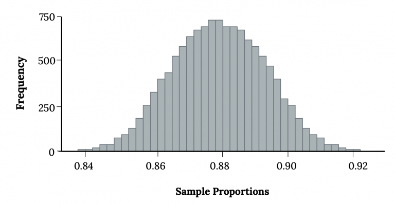
A histogram of the sampling distribution of the sample proportion with a smooth normal curve superimposed, illustrating how repeated samples form an approximately normal pattern when conditions are met. Numerical labels shown represent just one simulation example and exceed syllabus requirements. Source.

Conditions for Normal Approximation

A central requirement for using the normal approximation comes directly from the syllabus specification: the approximation is appropriate only when both $np \ge 10$ and $n(1 - p) \ge 10$. These criteria ensure that the sampling distribution has enough observations in both the “success” and “failure” categories to avoid skewness or distortion.

Why These Conditions Matter

• The condition $np \ge 10$ ensures the expected number of successes is sufficiently large.

• The condition $n(1-p) \ge 10$ ensures the expected number of failures is also sufficiently large.

• Together, they guarantee that repeated samples will produce proportions centered around the true population proportion with variability that behaves predictably.

These criteria apply specifically to categorical variables, where outcomes can be classified into two categories—often called “successes” and “failures,” but applicable to any binary classification. When these conditions are met, the sampling distribution becomes symmetric enough for a normal curve to model it accurately.

Structure of the Sampling Distribution Under Normal Approximation

Even though students should not perform calculations in these notes, they should understand the components that shape the approximated distribution. Under the conditions stated above, the sampling distribution of p^\hat{p}p^​ is centered at the population proportion and has a predictable spread.

EQUATION

These expressions define the location and spread of the approximated normal curve. Once the distribution is approximated as normal, probability statements about the value of p^\hat{p}p^​ can be made by converting sample proportions to $z$-scores and finding associated areas under the standard normal curve.

A normal sentence is placed here to maintain proper formatting before the next block.

Understanding the Behavior of Sample Proportions

The sampling distribution of a sample proportion reflects the idea that statistics vary from sample to sample. Even when all samples come from the same population, randomness introduces natural variation. When the conditions are met and the normal approximation applies, this variation becomes structured enough to analyze using standard probability tools.

Key characteristics under normal approximation

• Center: The distribution is centered at the population proportion, meaning p^\hat{p}p^​ is an unbiased estimator.

• Spread: Larger samples reduce the standard deviation, making the sampling distribution tighter around the true value.

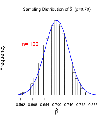
Three sampling distributions of the sample proportion for increasing sample sizes, each approximately normal. As sample size grows, the distributions narrow, demonstrating the decreasing standard deviation of p^\hat{p}p^​. Exact numerical labels are example-based and extend beyond syllabus requirements. Source.

• Shape: When the success–failure conditions are satisfied, the distribution becomes approximately bell-shaped, allowing the use of normal techniques.

These features support valid statistical reasoning about proportions, enabling students to judge how unusual or typical a sample result may be.

Using the Normal Approximation Responsibly

Although using the normal distribution greatly simplifies inference, it must be applied only when justified. Misapplication can lead to inaccurate probability statements or incorrect interpretations.

Essential safeguards

• Always verify the success–failure conditions before using the normal model.

• Recognize that skewed or small populations can distort the distribution when conditions are not met.

• Understand that the approximation improves as the sample size increases; borderline cases may still show slight asymmetry.

• Keep in mind that this approximation describes the distribution of the statistic, not the distribution of individual observations.

Interpretive Implications

Using the normal approximation allows students to translate questions about sample proportions into questions about areas under the normal curve. This makes it possible to evaluate how likely a sample proportion is, given the true population proportion, and to make inferential judgments about whether observed sample results are consistent with expectations.

Interpretation requires attention to context, units, and the connection between sample-level statistics and population-level parameters. When conditions permit, the normal approximation provides a reliable, intuitive framework for studying sampling variability in categorical settings.