The behavior of a sample proportion reveals how population characteristics manifest across repeated samples, helping students understand why sample results vary and how that variation can be modeled predictably.

Determining Parameters of Sampling Distributions for Sample Proportions

Understanding the parameters of the sampling distribution of a sample proportion is essential because these parameters describe how the statistic behaves across all possible random samples of the same size. For AP Statistics, the two key parameters are the mean of the sampling distribution and its standard deviation, each playing a different but complementary role in characterizing the distribution.

The Role of the Sample Proportion

A sample proportion, denoted $\hat{p}$, represents the proportion of individuals in a sample who exhibit a particular categorical characteristic. It serves as an estimate of a population proportion, denoted $p$, which measures the true proportion in the entire population. Because samples differ, sample proportions will vary from one sample to another, producing a predictable distribution when samples are independent and identically sized.

This sampling variation leads to a distribution whose center and spread reveal important information about how closely sample results cluster around the population truth.

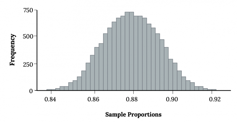
This histogram shows a simulated sampling distribution of the sample proportion centered near the population proportion ppp. The bell-shaped form reflects typical sampling variability when independence and sample-size conditions are met. Although the original source introduces normal approximation, here it visually supports understanding of the mean and standard deviation of the sampling distribution. Source.

Mean of the Sampling Distribution

The mean of the sampling distribution of $\hat{p}$ gives the long-run average of sample proportions over many random samples. According to the specification, this mean equals the true population proportion $p$, making the sample proportion an unbiased estimator of the population proportion.

EQUATION

This property ensures that, over repeated sampling, the average of all sample proportions will match the true parameter. This unbiasedness is a cornerstone of inferential methods that rely on sample proportions.

Standard Deviation of the Sampling Distribution

The standard deviation of $\hat{p}$ describes how much sample proportions vary from sample to sample. The syllabus specifies that when sampling with replacement, or when sampling without replacement from a large population, the standard deviation depends on the population proportion and the sample size.

EQUATION

Because proportions closer to 0.5 generate more variability and larger samples reduce variability, the formula reflects two intuitive principles:

• Populations with more balanced outcomes lead to more uncertain sample results.

• Larger samples stabilize estimates by averaging across more observations.

The 10% Condition and Sampling Without Replacement

While the standard deviation formula assumes sampling with replacement, real-world data collection often involves sampling without replacement. In these cases, observations are not perfectly independent, and the standard deviation should be slightly smaller. However, the specification states that this difference is negligible when the sample size is less than 10% of the total population size.

This condition supports the continued use of the same standard deviation formula in practical settings such as surveys, experiments, and observational studies where the population is large relative to the sample.

Ensuring Independence and Appropriate Use

For the formulas and interpretations to hold, the samples must meet the condition of independence. This arises naturally when:

• Sampling is conducted with replacement, or

• Sampling is without replacement but the 10% condition is satisfied.

Independence ensures that the behavior of one sampled individual does not meaningfully influence another, preserving the theoretical properties of the sampling distribution.

Why These Parameters Matter

Knowing the mean and standard deviation of the sampling distribution of $\hat{p}$ enables students to:

• Predict how much variation to expect in sample results

• Assess how typical or unusual certain sample proportions are

• Understand why different samples produce different estimates even when drawn from the same population

• Prepare for later topics involving normal approximations, confidence intervals, and hypothesis testing

The parameters articulate both the expected value of a sample proportion and the level of uncertainty associated with sampling. These insights form the backbone of statistical reasoning involving categorical data.

Key Takeaways for AP Statistics

• The sample proportion is an unbiased estimator of the population proportion.

• The variability of $\hat{p}$ decreases as sample size increases.

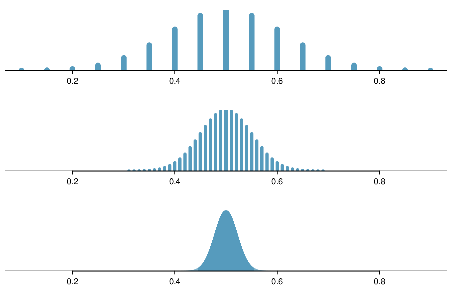
This figure displays sampling distributions of p^\hat pp^​ for increasing sample sizes nnn, illustrating the decreasing spread predicted by the formula for σp^\sigma_{\hat p}σp^​​. As nnn grows, the distributions become narrower and more concentrated around the true proportion. The figure also shows the shape becoming more nearly normal, which is slightly beyond the scope of this subsubtopic but helpful for conceptual understanding. Source.

• The standard deviation formula applies under sampling with replacement or when the sample is less than 10% of the population.

• These parameters guide how we model and interpret sample-based estimates in real data settings.