Normal Approximation for Differences in Proportions (5.6.2) | AP Statistics Notes

AP Syllabus focus:
‘The sampling distribution of the difference in sample proportions (p̂1 - p̂2) can be approximated by a normal distribution if the sample sizes are large enough, specifically if np1, n(1-p1), np2, and n(1-p2) are all greater than or equal to 10 for both populations. This condition is crucial for the validity of normal approximation methods.’

This subsubtopic explains when the difference in sample proportions behaves enough like a normal distribution to justify probability calculations, enabling valid inference about two populations.

Normal Approximation for Differences in Proportions

When comparing two independent populations, statisticians often analyze the difference in sample proportions, written as p̂1 − p̂2, to make inferences about how two groups differ. Understanding when this statistic follows an approximately normal distribution is essential because many inferential methods rely on normal probability models.

Conditions for Normal Approximation

The AP syllabus emphasizes that normal approximation is appropriate only when specific size and success–failure conditions are met. These conditions ensure the sampling distribution of p̂1 − p̂2 is sufficiently symmetric and mound-shaped to approximate normality with confidence.

Before discussing these conditions, recall that a sample proportion is a statistic summarizing the proportion of individuals in a sample who exhibit a particular categorical outcome.

Sample Proportion (p̂): The number of individuals in the sample with a specified categorical outcome divided by the total sample size.

When comparing proportions from two independent samples, the statistic of interest becomes the difference between them. This difference helps quantify how much more or less common an outcome is in one population relative to another.

To use the normal distribution to model the sampling distribution of p̂1 − p̂2, AP Statistics requires verifying the following conditions:

Independence Within Each Sample
- Sampling must be independent within each population.
- When sampling without replacement, each sample should be less than 10% of its population.
Independence Between Samples
- The two samples must come from distinct, non-overlapping populations or represent independent groups.
Success–Failure Condition for Both Samples
Each sample must contain enough expected successes and failures:
- n₁p₁ ≥ 10
- n₁(1 − p₁) ≥ 10
- n₂p₂ ≥ 10
- n₂(1 − p₂) ≥ 10

This set of requirements ensures that each sample proportion is approximately normal, which then guarantees that their difference is also approximately normal.

When these conditions are met, the distribution of p̂1 − p̂2 becomes smooth and symmetric, with most values clustering near the true difference p1 − p2.

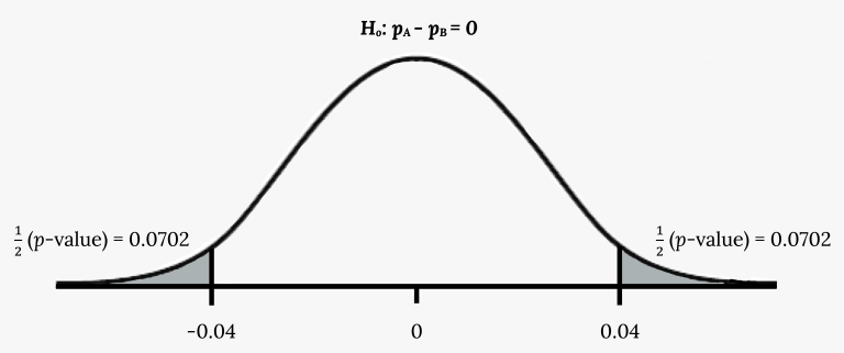
This graph displays a normal distribution for the difference in sample proportions, centered at a mean difference of zero. The shaded tails represent unusually large positive or negative differences that would have small probabilities under the normal model. Although the shading is shown in the context of a hypothesis test, the same curve shape represents the approximate sampling distribution of p̂₁ − p̂₂ when the normal approximation is valid. Source.

Why These Conditions Matter

Normal approximation hinges on the idea that both sample proportions stabilize toward predictable distributions when sample sizes are sufficiently large. When these conditions are met, the distribution of p̂1 − p̂2 becomes smooth and symmetric, with most values clustering near the true difference p1 − p2. This makes the normal model a reliable tool for reasoning about probabilities and variability.

Without the success–failure criteria, the distribution of sample proportions may be skewed or irregular. In such cases, using a normal distribution could produce misleading probability statements or inaccurate inferential conclusions.

Mean and Standard Deviation of the Sampling Distribution

When conditions for normal approximation are satisfied, the sampling distribution of the difference in sample proportions is centered around the true population difference and has a calculable spread. Understanding how these parameters behave helps justify normal approximation under the required conditions.

EQUATION

$\mu_{p̂_1 - p̂_2} = p_1 - p_2$
$\mu$ = Mean of the sampling distribution

$\sigma_{p̂_1 - p̂_2} = \sqrt{\frac{p_1(1 - p_1)}{n_1} + \frac{p_2(1 - p_2)}{n_2}}$
$\sigma$ = Standard deviation of the sampling distribution
$n_1, n_2$ = Sample sizes for populations 1 and 2
$p_1, p_2$ = True population proportions

These expressions rely on the independence and success–failure conditions discussed earlier. Without those conditions, the mean and standard deviation formulas may not accurately describe the behavior of the statistic.

The structure of the standard deviation formula highlights how variability decreases with larger sample sizes. As sample sizes increase, each term in the denominator grows, causing the overall spread of the sampling distribution to shrink.

As sample sizes increase, each term in the denominator grows, causing the overall spread of the sampling distribution to shrink.

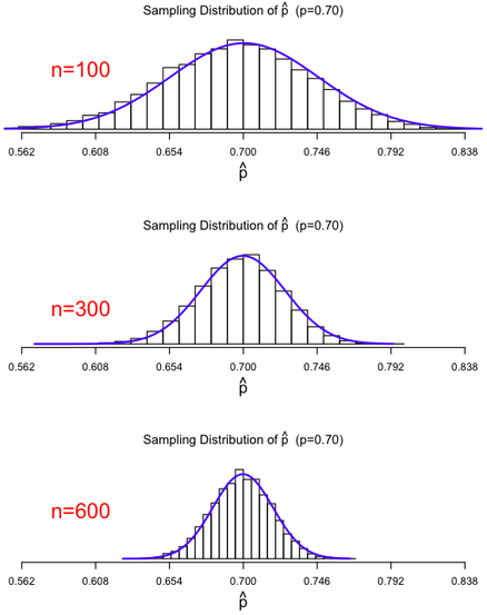
These three histograms show the sampling distribution of a sample proportion p̂ for increasing sample sizes, each overlaid with a smooth normal curve. As n grows, the distribution becomes more symmetric and narrow, illustrating why large samples produce a better normal approximation and smaller standard deviation. Although the figure displays a single-proportion scenario, the same idea explains why the sampling distribution of p̂₁ − p̂₂ becomes more normal and less variable as both sample sizes increase. Source.

Practical Interpretation of Conditions

To determine whether the normal approximation is justified in real problems, students must verify the required conditions systematically. A thorough check involves:

Identifying each population proportion, or using sample estimates if population values are unknown in practice.
Calculating the expected number of successes and failures for each sample.
Confirming independence, often through sampling procedures or contextual information.
Ensuring both samples meet all requirements before applying a normal model.

Benefits of Meeting Normal Approximation Conditions

When all conditions hold, the normal approximation enables powerful inferential techniques. It permits the use of z-scores and normal probability calculations to reason about the likelihood of observed differences or to construct confidence intervals for p1 − p2. These procedures form the backbone of comparing proportions across populations, making mastery of these conditions essential for AP Statistics students.

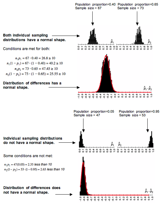
This figure contrasts situations in which the sampling distributions of individual sample proportions are or are not well approximated by normal curves, and shows how that affects the shape of the distribution of p̂₁ − p̂₂. It highlights that the normal approximation for the difference is appropriate only when both individual sampling distributions satisfy the success–failure conditions. The figure includes some extra contextual labeling, but its main message concerns when the normal model can be applied. Source.

FAQ

When proportions fall near the extremes of 0 or 1, even large samples may struggle to meet the success–failure criteria. This is because one of the expected counts becomes very small.

In such cases, the normal approximation becomes unreliable, and alternative methods such as randomisation tests or exact binomial procedures are preferred.

If samples are not independent, outcomes in one group may influence those in the other, which distorts the variability of the difference in sample proportions.

Independence ensures the variance formula for p̂1 − p̂2 remains valid. Without it, the spread of the sampling distribution could be underestimated or overestimated, making probability statements and inference inaccurate.

Not necessarily. Improvement depends on each group’s sample size and underlying proportion.

A group with a moderate proportion (around 0.5) requires a smaller sample for normality, while a group with a very small or very large proportion may require a substantially larger sample to satisfy success–failure conditions.

The normal approximation should not be used. Both sample proportions must individually satisfy the conditions for the difference to follow an approximately normal distribution.

This is because the shape of the combined distribution depends on the behaviour of both component sampling distributions. One poorly behaved sample can distort the overall distribution of p̂1 − p̂2.

Larger samples reduce the influence of random fluctuations in the counts of successes and failures.

Because both sample proportions approach normality with increasing n, their difference inherits this symmetry, producing a smoother, more bell-shaped distribution that aligns well with the normal model used in inference.

Practice Questions

Question 1 (1–3 marks)
A researcher takes two independent random samples to compare the proportion of adults who prefer Product A in Region 1 and Region 2. The sample sizes are n1 = 80 and n2 = 75. The estimated population proportions are p1 = 0.35 and p2 = 0.44.

Determine whether the normal approximation for the sampling distribution of p̂1 − p̂2 is appropriate. Justify your answer using the success–failure conditions.

Question 1 (1–3 marks)
• 1 mark for correctly calculating expected successes and failures in Region 1 (n1p1 = 28, n1(1–p1) = 52).
• 1 mark for correctly calculating expected successes and failures in Region 2 (n2p2 = 33, n2(1–p2) = 42).
• 1 mark for concluding that all values are at least 10 and therefore the normal approximation is appropriate.

Question 2 (4–6 marks)
A school wishes to compare the proportions of Year 12 students and Year 13 students who plan to apply to university. A random sample of 150 Year 12 students finds that 96 intend to apply. A separate random sample of 140 Year 13 students finds that 112 intend to apply.

(a) State the sample proportions for each year group.
(b) Verify whether the conditions for using a normal approximation for the sampling distribution of p̂1 − p̂2 are satisfied.
(c) Explain why meeting these conditions is necessary before constructing a confidence interval for the difference in population proportions.

Question 2 (4–6 marks)

(a)
• 1 mark for correct Year 12 sample proportion: 96/150 = 0.64.
• 1 mark for correct Year 13 sample proportion: 112/140 = 0.80.

(b)
• 1 mark for correctly checking expected successes and failures for Year 12 (96 successes, 54 failures; both ≥ 10).
• 1 mark for correctly checking expected successes and failures for Year 13 (112 successes, 28 failures; both ≥ 10).
• 1 mark for concluding that the normal approximation is appropriate because all conditions (including independence) are met.

(c)
• 1 mark for explaining that the sampling distribution must be approximately normal for standard confidence interval methods to be valid.
• 1 mark for stating that without normality, probability statements and margin-of-error calculations may be inaccurate.

Try All Topic Practice Questions

Written by:

Dr Rahil Sachak-Patwa

Oxford University - PhD Mathematics

Rahil spent ten years working as private tutor, teaching students for GCSEs, A-Levels, and university admissions. During his PhD he published papers on modelling infectious disease epidemics and was a tutor to undergraduate and masters students for mathematics courses.