Understanding how to interpret probabilities and parameters for the sampling distribution of a difference in sample proportions is essential for making context-rich, meaningful inferences about populations.

Interpreting Parameters of the Sampling Distribution

When comparing two population proportions, the sampling distribution of the difference in sample proportions—written as $\hat{p}_1 - \hat{p}_2$—provides a model for how this statistic behaves across repeated random samples. To interpret this distribution correctly, students must recognize how each parameter links back to the populations being studied and what each probability statement communicates about expected sampling outcomes.

Interpreting the sampling distribution of p^1−p^2\hat{p}_1 - \hat{p}_2p^​1​−p^​2​ means thinking of all the differences we could have seen over many random samples, not just the one we actually observed.

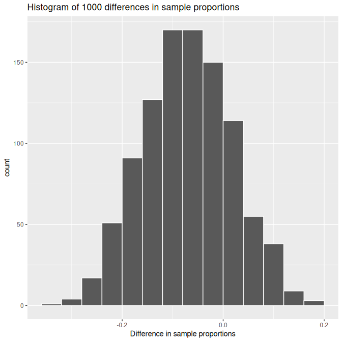
Histogram of 1,000 simulated differences in sample proportions across repeated samples. The distribution shows how values of p^1−p^2\hat p_1 - \hat p_2p^​1​−p^​2​ cluster around the center with natural sampling variability. The specific red-ball/almond context in the original source exceeds AP requirements, but the statistical structure exactly matches the sampling distribution principles described in these notes. Source.

Mean of the Sampling Distribution

The mean of the sampling distribution describes the average value of $\hat{p}_1 - \hat{p}_2$ over all possible samples of the same sizes.

EQUATION

This parameter must always be interpreted within the context of the specific populations, emphasizing that it reflects the underlying difference in true proportions, not the difference observed in one sample. Recognizing this distinction helps separate population-level reality from sample-level variability.

Interpreting this parameter requires precise language. For example, stating that the mean equals $p_1 - p_2$ communicates that, on average, repeated samples would yield a difference in sample proportions equal to the actual difference in the population.

Standard Deviation of the Sampling Distribution

The standard deviation of the sampling distribution describes the expected variability of $\hat{p}_1 - \hat{p}_2$ across repeated sampling. It communicates how much fluctuation should naturally occur from sample to sample.

EQUATION

The interpretation must emphasize both units (proportions) and context. Saying that the standard deviation is, for example, 0.04 is incomplete without clarifying that it represents the expected typical deviation in the difference in sample proportions when repeatedly sampling from the two populations.

Interpreting Probabilities Associated with the Distribution

Probability statements for $\hat{p}_1 - \hat{p}_2$ quantify how likely it is for samples to produce differences of various magnitudes. Proper interpretation requires clearly identifying the populations, the parameter of interest, and the direction and meaning of inequalities.

Contextual Interpretation of Probability Statements

When interpreting a probability such as

• “The probability that $\hat{p}_1 - \hat{p}_2$ exceeds 0.10,”
  the student must connect this to the likelihood of obtaining a sample difference at least that large when sampling from the two specified populations.

Important elements to highlight include:

• the specific populations and the categorical variables involved

• the fact that probabilities refer to random samples, not individuals

• understanding that probabilities describe outcomes under repeated sampling, not certainty about a single observed difference

Using Proper Units and Comparative Language

Interpretation must reflect that differences in proportions represent comparisons. Students should use phrasing such as:

• “Population 1 has a higher proportion of ___ than Population 2,”
  or

• “The sample difference suggests that, in repeated sampling, differences of this magnitude occur with probability ___.”

Avoiding vague statements (e.g., “there is a difference”) is essential. Instead, the interpretation must specify which population has the higher proportion and by how much.

Connecting Parameters and Probabilities to Real-World Meaning

When the normal approximation is valid, the probability for a range of values of p^1−p^2\hat p_1 - \hat p_2p^​1​−p^​2​ is represented by the area under a normal curve between the corresponding boundaries.

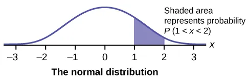
Standard normal curve with the area between one and two standard deviations shaded. This illustrates how probabilities for continuous statistics such as p^1−p^2\hat p_1 - \hat p_2p^​1​−p^​2​ or their z-scores correspond to areas under the curve. The exact numerical boundaries (1 and 2) exceed what the syllabus requires but provide a clear visual model for probability interpretation. Source.

Emphasizing Context

Every interpretation should return to the real-world populations being studied. Without context, numerical results lack meaning. Students should be trained to:

• name the populations explicitly

• name the characteristic being compared

• state conclusions in terms of proportions, not counts or percentages of samples

Understanding Variability Across Samples

Because the sampling distribution models how $\hat{p}_1 - \hat{p}_2$ varies, interpretations must acknowledge sampling variability. Proper interpretation might include statements such as:

• “Differences in sample proportions will vary from sample to sample,”
  or

• “A difference of this size is typical/atypical under repeated sampling.”

This reinforces the statistical reasoning that conclusions are based not on single samples but on modeled sampling behavior.

Interpreting Extremely Large or Small Differences

Students should recognize that unusually large observed differences (relative to the distribution’s mean and standard deviation) may suggest that:

• random sampling variability alone may not explain the result

• there may be a meaningful difference between population proportions

However, interpretations should not extend into hypothesis-testing territory; the focus remains on understanding what probabilities and parameters mean, not on conducting formal inference.

Layered Interpretation Checklist

Students can approach interpretation systematically by ensuring that statements include:

• Context

  • Name each population.

  • Describe the categorical variable.

• Parameter clarity

  • Identify the population difference being estimated.

• Statistic clarity

  • Define the sample difference being described.

• Probability interpretation

  • Express likelihood in terms of repeated sampling.

• Units

  • Use proportion differences, not percentages of individuals.

This layered approach supports consistent, precise interpretation of both parameters and probabilities associated with the sampling distribution for differences in sample proportions.