Determining Parameters for Differences in Proportions (5.6.1) | AP Statistics Notes

AP Syllabus focus:
‘For two independent populations with population proportions p1 and p2, when sampling with replacement, the sampling distribution of the difference in sample proportions (p̂1 - p̂2) has mean μ(p̂1 - p̂2) = p1 - p2 and standard deviation σ(p̂1 - p̂2) = sqrt[(p1(1-p1)/n1) + (p2(1-p2)/n2)]. If sampling without replacement and the sample sizes are less than 10% of the population sizes, the standard deviation's adjustment for the finite population correction is negligible.’

When comparing two groups using categorical data, understanding the behavior of the difference in sample proportions is essential for making reliable inferences about real population differences. These parameters describe how sample results vary.

Understanding the Sampling Distribution for Differences in Proportions

The sampling distribution of $\hat{p}_1 - \hat{p}_2$ describes all possible values of the difference between two sample proportions when repeatedly sampling from two independent populations. This distribution provides the foundation needed to evaluate whether observed differences in sample outcomes reflect real population differences or random sampling variation.

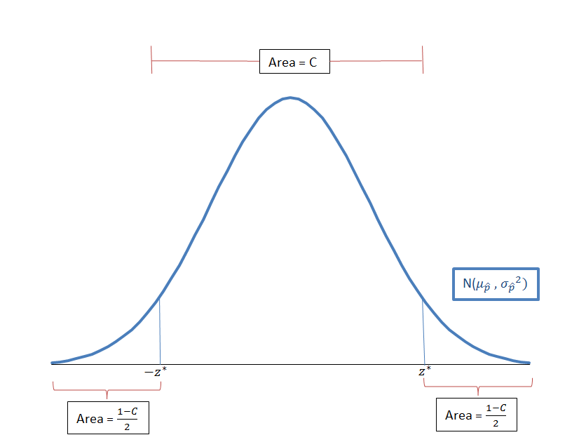
A bell-shaped sampling distribution of sample proportions, illustrating how a statistic varies across many repeated samples from the same population. The same conceptual structure underlies the sampling distribution of the difference in sample proportions. The image contains no extraneous information beyond the core distribution shape. Source.

Because sampling involves chance, the statistic $\hat{p}_1 - \hat{p}_2$ will vary from sample to sample. Quantifying this variability requires determining the distribution’s center (mean) and spread (standard deviation). These parameters allow the distribution to be approximated and used for inference in later topics.

Independence and Sampling With Replacement

When developing parameters of this sampling distribution, AP Statistics assumes sampling with replacement unless otherwise stated. This assumption guarantees independence between individual observations. Independence is important because the formulas for variability rely on the idea that each observation provides unique information unrelated to others.

If sampling occurs without replacement, independence no longer holds perfectly. However, when each sample size is less than 10% of its population, the loss of independence is negligible. This is commonly known as the 10% condition, and it allows the standard formulas for variability to be used without adjustment.

Mean of the Sampling Distribution

The mean of the sampling distribution of the difference in sample proportions reflects the true difference in population proportions. Because each sample proportion is an unbiased estimator of its population proportion, their difference is also unbiased.

EQUATION

$\mu_{\hat{p}_1 - \hat{p}_2} = p_1 - p_2$
$p_1$ = Population proportion for group 1
$p_2$ = Population proportion for group 2

This mean represents the expected difference between sample proportions if many samples were taken. It provides the central value around which sample differences vary.

Understanding the center of this distribution is crucial because it links sample outcomes to population parameters, making the distribution a powerful inferential tool.

Standard Deviation of the Sampling Distribution

The standard deviation measures the spread of the distribution and reflects how much the difference in sample proportions is expected to vary from sample to sample. More variability in either group’s population proportion or smaller sample sizes increases this spread.

EQUATION

$\sigma_{\hat{p}_1 - \hat{p}_2} = \sqrt{\frac{p_1(1-p_1)}{n_1} + \frac{p_2(1-p_2)}{n_2}}$
$n_1$ = Sample size for group 1
$n_2$ = Sample size for group 2

This formula applies when sampling with replacement or when the 10% condition is met. It reflects the combined variability from both samples. A larger sample size reduces variability, stabilizing the estimate.

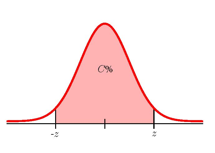
A normal distribution diagram marking –z and z with the central C% region shaded. It visually represents the model used for inference involving two proportions. The inclusion of the C% confidence label reflects material slightly beyond the parameters subsubtopic but still directly tied to the same sampling distribution structure. Source.

Between equation and definition blocks, we maintain clear explanatory text. The standard deviation plays a vital role because it determines how widely sample results may differ, guiding the interpretation of observed sample differences.

Components Affecting Variability

Several structural elements influence the standard deviation of $\hat{p}_1 - \hat{p}_2$ :

Sample Sizes

Larger $n_1$ or $n_2$ reduce the standard deviation because individual sample proportions become more stable with more data.

Population Proportions

The expressions $p(1-p)$ represent variability in binary outcomes. When proportions approach 0.5, variability is highest; when they approach 0 or 1, variability decreases.

Independence

Independence between populations ensures no overlap in membership or influence between groups, maintaining the validity of the variance formula.

Key Conditions for Using These Parameters

To correctly determine the parameters of the sampling distribution of $\hat{p}_1 - \hat{p}_2$ , AP students must confirm:

Two independent populations
Independence must exist both between and within samples.
Sampling with replacement, or the 10% condition must hold
This preserves approximate independence of observations.
Correct identification of population proportions and sample sizes
These values directly feed into the formulas for mean and standard deviation.

Why These Parameters Matter

Understanding these parameters provides the essential foundation for later inference procedures involving two proportions, including confidence intervals and significance tests. The mean identifies the central expected difference, while the standard deviation quantifies typical variation in sample outcomes. These components together describe how sample evidence reflects true population differences, forming a cornerstone of statistical reasoning in comparative categorical analysis.

FAQ

When p1 and p2 are close together, the mean of the sampling distribution (p1 minus p2) will be near zero, indicating little expected difference between samples.

However, the variability remains determined by the size of each sample and the variability within each population. Even small true differences can produce noticeable sample differences when sample sizes are small or when the proportion variability is high.

Large samples help stabilise the estimate, making small underlying differences easier to detect.

Yes. The two sample sizes independently affect the total variability.

• A larger n reduces the contribution of its group’s variability.
• If one sample is much larger than the other, the smaller sample dominates the overall spread.
• The sampling distribution will still be centred at p1 minus p2, but its spread will reflect the imbalance in precision between groups.

Different sample sizes do not change the mean, only the spread and reliability of estimates.

Independence ensures that the variability in one group does not influence the variability in the other.

If the samples overlap or the groups affect each other, the formula for standard deviation no longer accurately reflects total variability. This can occur when the same individuals appear in both samples or when the groups interact in a way that changes response probabilities.

Maintaining independence guarantees that the contributions to variability come from distinct sources.

When a population proportion is near 0 or 1, its term p(1 – p) becomes very small, reducing that group’s contribution to the overall variability.

As a result:
• The standard deviation of the difference in sample proportions becomes smaller.
• The distribution becomes more narrowly concentrated around its mean.
• The difference p1 minus p2 may still be large or small, but it will be estimated more precisely for that group.

This effect reflects reduced uncertainty when outcomes are nearly uniform.

Sampling with replacement guarantees independence between individuals, which keeps the probability structure stable across selections.

It also simplifies the theoretical development of the sampling distribution, ensuring that each draw reflects the true population proportion without depletion.

In practical settings where sampling without replacement is common, the theory still applies as long as the 10% condition holds, allowing the simpler formulas to remain accurate while avoiding complex finite population corrections.

Practice Questions

Question 1 (1–3 marks)
A researcher compares two independent groups. In Group A, the population proportion of students who prefer online quizzes is 0.62. In Group B, the population proportion is 0.55. Samples of size 80 from each group are taken with replacement.
State the mean of the sampling distribution of the difference in sample proportions (p-hat A – p-hat B), and explain what this mean represents in context.

Question 1 (1–3 marks)
• 1 mark: Correctly states the mean as 0.62 – 0.55 = 0.07.
• 1 mark: Identifies that this value is the expected difference in sample proportions across many repeated samples.
• 1 mark: Provides a contextual explanation (e.g., on average, sample proportions from Group A will exceed those from Group B by about 0.07 if many samples are taken).

Question 2 (4–6 marks)
A school is investigating whether the proportion of students who complete homework on time differs between Year 10 and Year 11. The true population proportion for Year 10 is 0.74 and for Year 11 is 0.68. Independent random samples of 60 students are selected from each year group, with sampling carried out with replacement.
(a) Calculate the standard deviation of the sampling distribution of the difference in sample proportions (Year 10 minus Year 11).
(b) Explain why the standard deviation formula used is appropriate for this situation.
(c) Interpret the meaning of this standard deviation in the context of the school.

Question 2 (4–6 marks)
(a)
• 1 mark: Correct substitution into the standard deviation formula using the values 0.74, 0.68, and sample size 60.
• 1 mark: Correct calculation of the standard deviation (approximately 0.083).

(b)
• 1 mark: States that sampling is with replacement or that observations can be treated as independent.
• 1 mark: States that both samples are independent groups.

(c)
• 1 mark: Provides an interpretation in context, referring to variation in the difference in sample proportions across repeated sampling.
• 1 mark: Makes clear that the standard deviation describes typical sampling variation, not individual student behaviour.

Try All Topic Practice Questions

Written by:

Dr Rahil Sachak-Patwa

Oxford University - PhD Mathematics

Rahil spent ten years working as private tutor, teaching students for GCSEs, A-Levels, and university admissions. During his PhD he published papers on modelling infectious disease epidemics and was a tutor to undergraduate and masters students for mathematics courses.