Understanding when the sampling distribution of the sample mean becomes approximately normal is essential for making valid probability statements about sample means in practical statistical investigations.

Normality Criteria for Sampling Distributions

The sampling distribution of the sample mean, often written as x-bar, plays a key role in inference. This subsubtopic focuses on how the shape of the population distribution and the size of the sample determine whether the sampling distribution of x-bar can be treated as approximately normal. These criteria allow students to apply normal probability methods appropriately in real data contexts.

Normal Population Distributions

When the underlying population is itself normally distributed, the sampling distribution of the sample mean is also normal for any sample size.

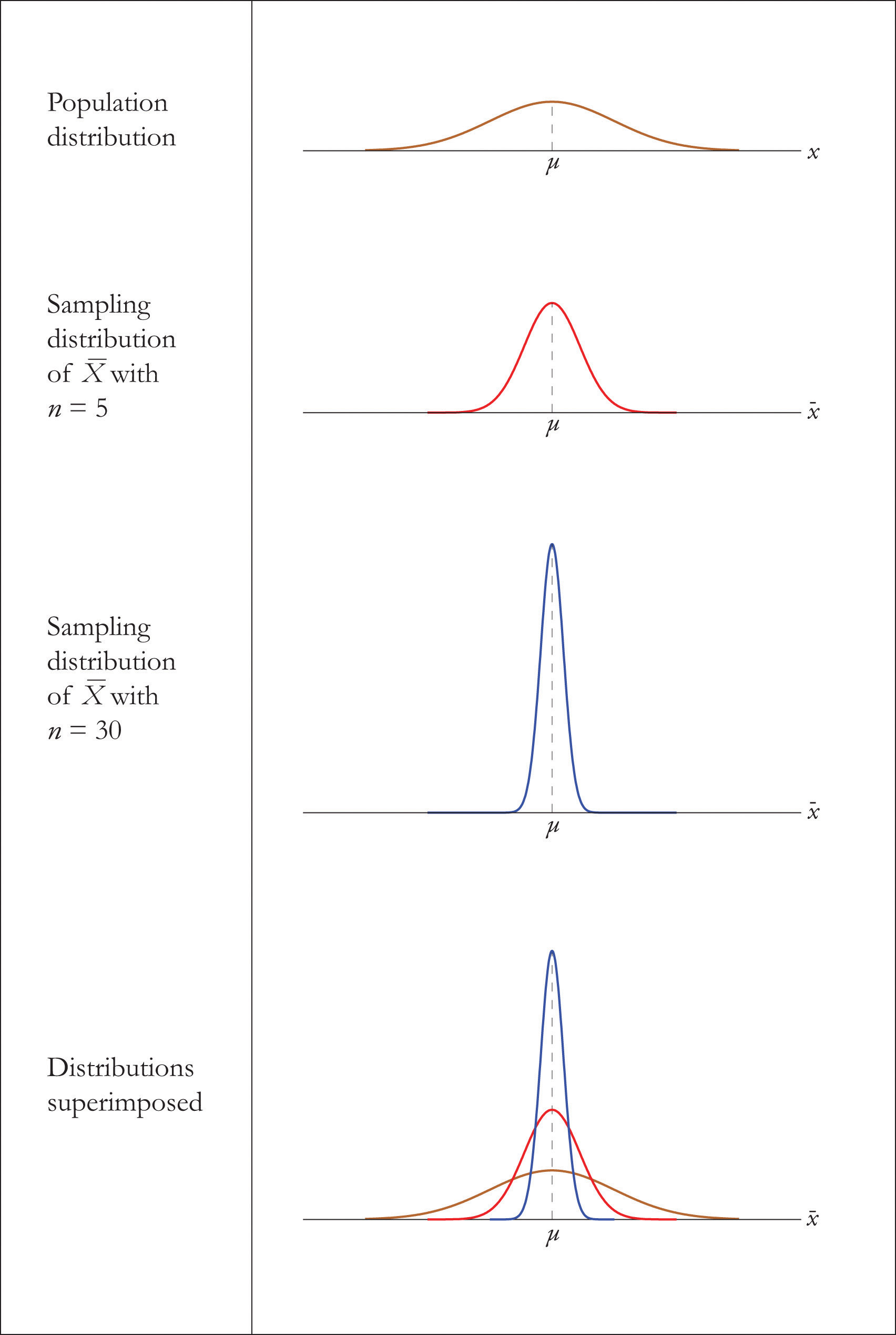
The figure illustrates how sampling distributions of the sample mean maintain a normal shape when drawn from a normal population and become narrower as sample size grows. Source.

This result holds whether the sample is small or large because the sample mean of values drawn from a normal population inherits normality from that population.

This property ensures that normal probability techniques can always be used for sample means when the population distribution is known to be normal. Students should recognize that this scenario provides the strongest guarantee of normality in sampling distributions.

Non-Normal Population Distributions

Many real-world populations are not well modeled by a normal distribution. They may be skewed, uniform, bimodal, or heavy-tailed. In such cases, the sampling distribution of the sample mean does not begin as normal for small sample sizes. Instead, its behavior depends on the Central Limit Theorem (CLT).

The CLT provides the foundation for using normal approximations even when the population distribution deviates substantially from normality.

Sample Size Requirements

For non-normal population distributions, the normal approximation improves as the sample size grows.

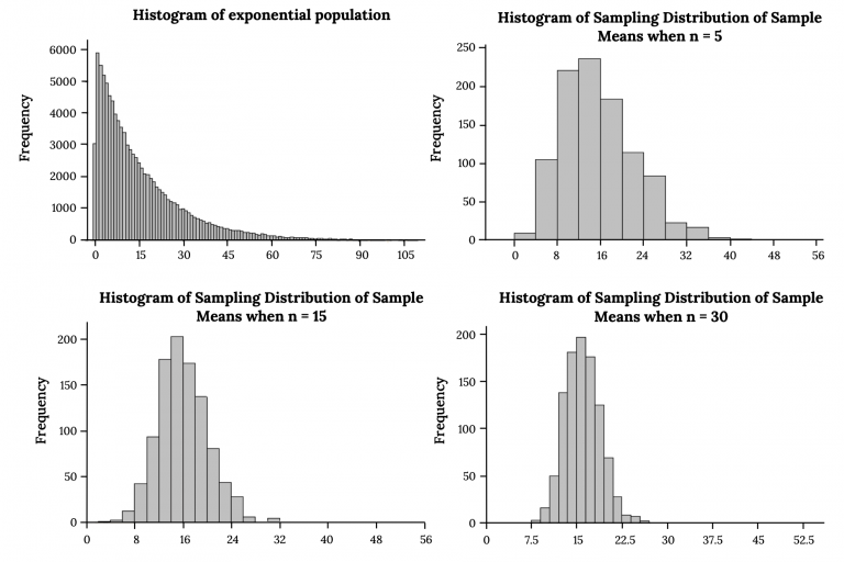
The figure demonstrates how sampling distributions of the mean become increasingly symmetric and approximately normal as sample size grows, even when the population itself is strongly skewed. Source.

The syllabus identifies n ≥ 30 as a commonly accepted threshold for the CLT to produce an approximately normal sampling distribution of x-bar.

Important points about the n ≥ 30 rule:

• It is a rule of thumb, not a strict mathematical boundary.

• It performs best when the population distribution is not extremely skewed.

• Larger samples may be required when the population contains strong skewness or outliers.

Students should learn to connect the shape of the population with the expected behavior of the sampling distribution as sample size changes.

Why the CLT Enables Normal Approximation

The Central Limit Theorem explains that as sample size increases, the influence of individual extreme values weakens. Each sample mean aggregates many observations, causing the distribution of these means to become smoother and more concentrated around the population mean.

This behavior supports the use of normal probability methods in many data analysis contexts, even when the population distribution is unknown or irregular, provided that the sample is sufficiently large.

Standard Deviation of the Sampling Distribution

Although this subsubtopic focuses on conditions for normality, students must remember that the shape of the sampling distribution interacts with its spread. The standard deviation of x-bar, often called the standard error, influences how quickly the distribution becomes tightly clustered around the mean as sample size increases.

EQUATION

This reduction in spread helps the distribution of sample means stabilize, reinforcing the normal shape predicted by the CLT for sufficiently large n.

A sentence here ensures proper spacing before further structured content.

Applying Normality Criteria in Practice

When determining whether it is appropriate to assume a normal sampling distribution for x-bar, students should consider:

• Population Shape

  • If the population is normal, the sampling distribution is normal for all n.

  • If the population is non-normal, normality depends on sample size.

• Sample Size

  • Use the normal model when n ≥ 30, unless the population distribution is extremely skewed.

  • Use caution with small samples from non-normal populations.

• Purpose of the Analysis

  • Probability calculations for x-bar require an approximately normal sampling distribution.

  • The validity of confidence intervals and hypothesis tests depends on meeting these criteria.

Key Takeaways for AP Students

To effectively apply normal probability techniques:

• Recognize when the shape of the population guarantees normality.

• Evaluate whether the sample size is sufficiently large for the CLT to apply.

• Use the normal distribution confidently when conditions are satisfied.

• Understand that these criteria are fundamental for the proper use of inference methods involving sample means.

These criteria form one of the central building blocks for statistical inference, enabling meaningful interpretation of sample means across varied population contexts.