This subsubtopic explains how the sampling distribution of the sample mean behaves, emphasizing how its center and spread relate to the population it comes from. Understanding these parameters is essential for interpreting sample data accurately.

Parameters of the Sampling Distribution of the Sample Mean

The concept of a sampling distribution forms the foundation for modern statistical inference. When many samples of the same size are repeatedly drawn from a population, the sample means form their own distribution.

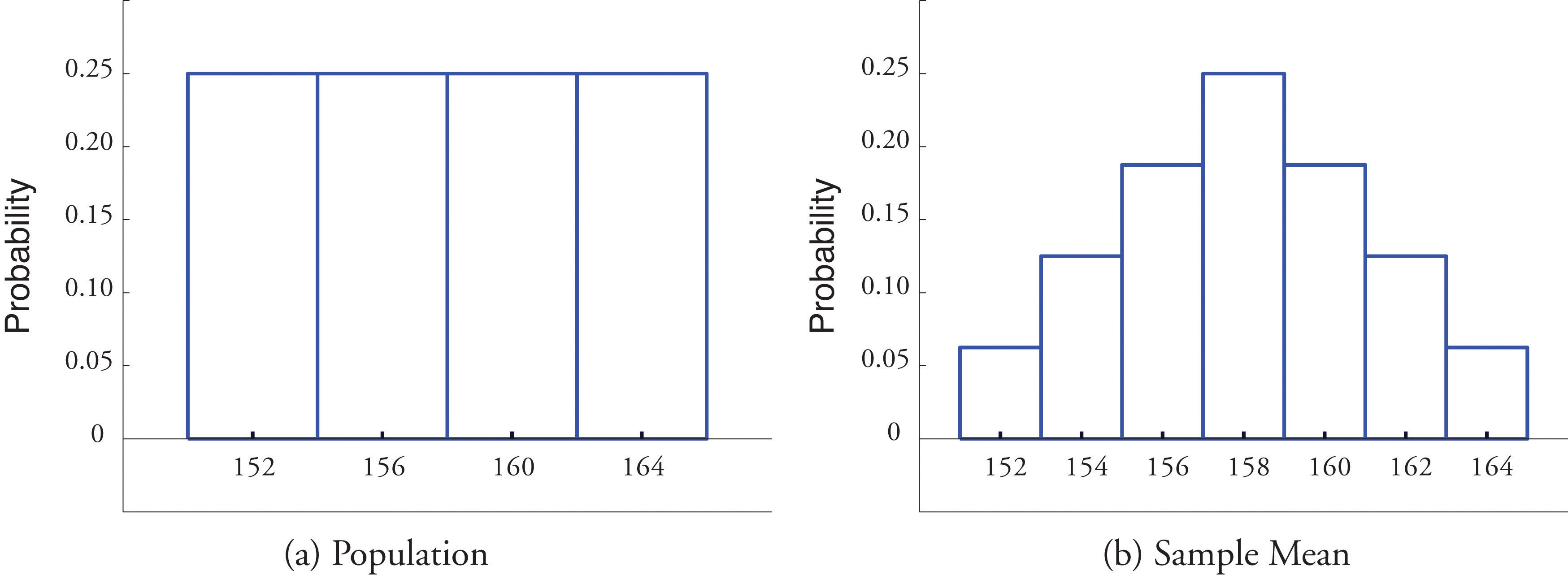
This figure contrasts the distribution of the population with the distribution of the sample mean for repeated samples. The sampling distribution is more concentrated around the center than the population distribution, illustrating that sample means vary less than individual data values. Its emerging bell shape reflects the structure that later connects to the Central Limit Theorem, though that concept extends beyond this subsubtopic. Source.

This distribution is predictable and structured, allowing statisticians to quantify uncertainty, compare samples, and perform formal inference procedures.

Understanding the Mean of the Sampling Distribution

The sampling distribution of the sample mean, often written as x̄, has a special and powerful property: its center is the same as the population’s true mean. This makes the sample mean a particularly useful and trustworthy estimator.

Because the average of all possible sample means equals the population mean, the sample mean is considered an unbiased estimator. This unbiasedness ensures that with repeated sampling, the estimator does not systematically overestimate or underestimate the true parameter.

EQUATION

This relationship tells us that, on average, x̄ targets the true population mean, which is essential for reliable inference.

A key implication is that increasing the sample size does not change the center of the sampling distribution. It only affects the spread, which determines how much the sample mean fluctuates between samples.

Understanding the Standard Deviation of the Sampling Distribution

The standard deviation of the sampling distribution, also known as the standard error of the mean, describes the variability of sample means across repeated samples. It quantifies how much the sample mean typically differs from the population mean.

When sampling with replacement—or when the sample is small relative to the population—the standard error has a consistent mathematical form. This form shows that larger samples reduce the variability of the sample mean, making estimates more precise.

EQUATION

This equation reveals several critical principles:

• Larger samples lead to smaller standard errors.

• Smaller standard errors mean more consistent sample means.

• A population with more variability (larger σ) produces more variable sample means.

• The square-root structure reflects diminishing returns: doubling the sample size does not halve the standard error, but reduces it by a factor of $\sqrt{2}$.

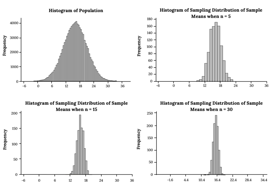
This figure displays a normal population alongside sampling distributions of the sample mean for several sample sizes. As the sample size increases, the sampling distributions become narrower while remaining centered at the same mean, illustrating the decreasing standard error. Its bell-shaped appearance reflects the behavior predicted by the Central Limit Theorem, which extends beyond this subsubtopic but connects naturally to later concepts in the syllabus. Source.

Understanding how the standard error behaves helps students evaluate reliability. When the standard error is small, a single sample mean is likely to be close to the population mean.

The Role of Population Size and Sampling Without Replacement

In many practical settings, sampling occurs without replacement. When a sample makes up more than 10% of the population, this has a noticeable impact on variability because values are not fully independent. However, the specification emphasizes that when:

• The sample size is less than 10% of the population,

the difference is negligible, allowing students to use the standard error formula without adjustment. This simplifies computations and aligns with typical AP Statistics practice.

Why These Parameters Matter

Understanding the parameters of the sampling distribution is essential because they:

• Support the logic behind statistical inference

• Connect the behavior of samples to the characteristics of populations

• Provide the foundation for confidence intervals and hypothesis tests

• Help students evaluate how reliable a single sample mean is as an estimate

Bullet points can help clarify core ideas students must retain:

• The mean of the sampling distribution equals the population mean.

• The standard deviation of the sampling distribution shrinks with larger sample sizes.

• Sampling with replacement or a sample smaller than 10% of the population ensures the standard error formula is valid.

• These parameters describe the predictable behavior of sample means across repeated samples.

The predictable structure of the sampling distribution allows statisticians to reason from samples to populations. Because the mean and standard error are known quantities, they form the mathematical backbone of the inferential procedures that follow in later topics.