Understanding when the difference in sample means behaves approximately normally is essential for conducting valid statistical inference and confidently applying normal distribution methods.

Normality of the Sampling Distribution for Differences in Sample Means

The sampling distribution of the difference in sample means, written as $\bar{x}_1 - \bar{x}_2$, is central to comparing two population means. Because inference procedures such as confidence intervals and significance tests for differences rely on normality, determining when this distribution is normal or approximately normal is an essential step in analysis. The syllabus highlights two primary conditions under which normality is guaranteed or reasonably approximated, depending on the characteristics of the populations and sample sizes involved.

When Both Populations Are Normally Distributed

When the two populations under study each follow a normal distribution, the sampling distribution of $\bar{x}_1 - \bar{x}_2$ is automatically normal, regardless of the sample sizes. The reason lies in the behavior of sample means: if population data are drawn from a normal distribution, then the sample mean is itself normally distributed for any sample size. Since the difference of two normally distributed variables is also normal, the resulting distribution of $\bar{x}_1 - \bar{x}_2$ satisfies normality without requiring large samples.

This feature allows researchers to conduct inference even with small samples, provided the population distributions are known to be normal. In practice, this situation is uncommon unless population shapes are well established or supported by strong contextual evidence.

When Populations Are Not Normally Distributed

In many real-world situations, populations are skewed, multimodal, or otherwise non-normal. In such cases, the sampling distribution of $\bar{x}_1 - \bar{x}_2$ does not begin normally. However, the Central Limit Theorem (CLT) provides a pathway to normality when sample sizes become sufficiently large.

A normal sentence must appear here to ensure proper separation from definition blocks.

The Role of Sample Size (n ≥ 30 Requirement)

The specification states that when populations are not normally distributed, both sample sizes must be at least 30 for the sampling distribution of the difference to be considered approximately normal.

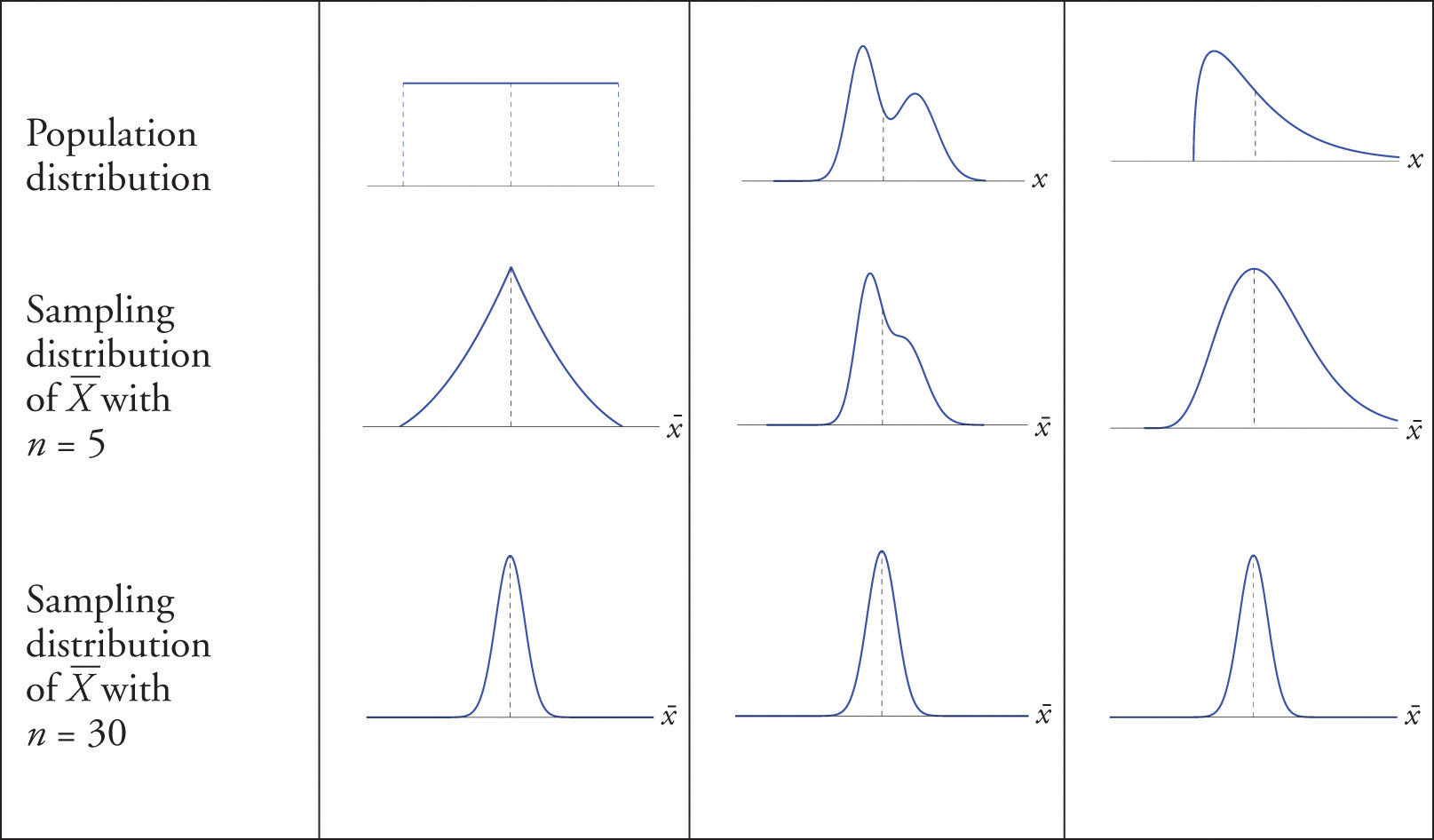
This figure compares a non-normal population to sampling distributions for different sample sizes, showing how larger samples produce more normal sampling distributions. Although drawn for a single sample mean, the same CLT logic applies to both sample means used when studying xˉ1−xˉ2\bar{x}_1 - \bar{x}_2xˉ1​−xˉ2​. Source.

Key reasons this condition matters include:

• Large samples reduce the influence of population skewness, causing the sampling distribution to smooth out.

• The distribution of the difference stabilizes only when each sample mean is itself well-approximated by a normal distribution.

• Normal approximation techniques, including $z$-procedures, require a reliable normal shape to ensure accurate probability interpretation.

When either sample is smaller than 30 and the population is strongly skewed, applying normal procedures becomes inappropriate without additional justification or alternative methods.

Why Normality Matters for Inference

Normality is not simply a theoretical preference—it determines the validity of commonly used inference tools. Whether constructing confidence intervals or conducting significance tests, analysts typically rely on the properties of the normal distribution to:

• Determine critical values

• Compute standardized test statistics

• Estimate tail probabilities

• Interpret variability in differences between sample means

Without normality or at least approximate normality, these procedures lose accuracy. Thus, verifying the conditions for normality is a required early step in any two-sample inference problem involving means.

A normal sentence belongs here to maintain the appropriate spacing before an equation box.

EQUATION

Practical Interpretation of the Normality Criteria

The criteria described in this subsubtopic guide students in determining when normal distribution methods are justified:

• If both populations are known or strongly supported to be normal, proceed with inference using any sample size.

• If population shapes are unknown or non-normal, ensure n₁ ≥ 30 and n₂ ≥ 30 before using normal procedures.

• Always verify independence and random sampling before evaluating normality conditions.

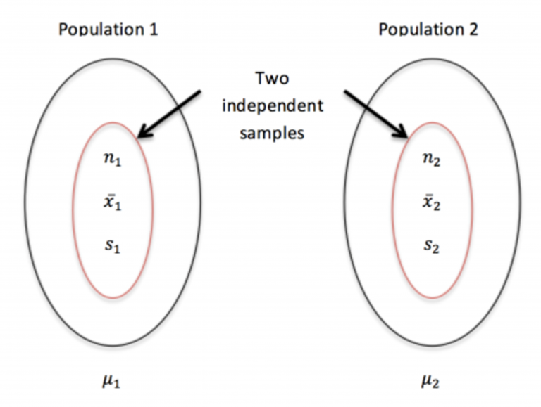
This illustration shows two independent samples drawn from separate populations, each producing its own sample mean. Independence of samples is a required condition before applying normality-based inference to the difference xˉ1−xˉ2\bar{x}_1 - \bar{x}_2xˉ1​−xˉ2​. Source.

These guidelines ensure that probability calculations involving $\bar{x}_1 - \bar{x}_2$ reflect the true behavior of repeated sampling and that resulting inferences about the difference in population means are statistically sound.