
AP Syllabus focus:
'When sampling with replacement from two independent populations with means (μ1 and μ2) and standard deviations (σ1 and σ2), the sampling distribution of the difference in sample means (x-bar1 - x-bar2) has a mean of (μ1 - μ2) and a standard deviation calculated by sqrt[(σ1^2/n1) + (σ2^2/n2)]. Adjustments for sampling without replacement are negligible if both sample sizes are less than 10% of their respective population sizes.'
Sampling distributions for differences in sample means help quantify how two independent samples may vary and provide a foundation for comparing population means using statistical inference.
Understanding Parameters of the Sampling Distribution
The difference in sample means is a statistic that measures how much two independent sample averages vary relative to each other.
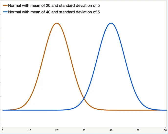
Two normal curves with equal spread but different centers illustrate populations with means μ₁ and μ₂, showing that the distance between their peaks represents the difference μ₂ − μ₁. This reinforces the idea that the mean of the sampling distribution of x̄₂ − x̄₁ equals the true difference in population means. No additional concepts beyond those in the notes are introduced. Source.
This statistic forms its own sampling distribution, which describes all possible values of the difference in sample means across all potential samples of the same size drawn from each population.
Sampling Distribution of a Statistic: The distribution of all possible values that a statistic can take when computed from every sample of a fixed size drawn from a population.
Because this subsubtopic focuses specifically on the difference in sample means, it is essential to understand how its center and spread are determined. These parameters allow us to anticipate the behavior of the statistic before observing real data.
Independence and Sampling With Replacement
The populations must be independent, meaning the outcome from one population provides no information about the other. This condition ensures that combining variances across samples is mathematically valid and interpretable. When sampling with replacement, each sample behaves as if drawn from an infinitely large population, making probability structures stable and consistent.
Mean of the Sampling Distribution
The mean of the sampling distribution of the difference in sample means reflects the true difference between the population means. Because sample means are unbiased estimators, the expected value of their difference equals the difference in population means.
EQUATION
= Population means for the two groups
This result tells us that, on average across many samples, the statistic x̄₁ − x̄₂ correctly centers around the true parameter μ₁ − μ₂.
Standard Deviation of the Sampling Distribution
The spread of the sampling distribution reflects how much the difference in sample means varies across repeated samples. Because the samples are independent, their variances add. Larger population variability or smaller sample sizes produce greater spread in the distribution.
EQUATION
= Population standard deviations
= Sample sizes
The standard deviation of the sampling distribution (also called the standard error of x̄₁ − x̄₂) combines the variability from both samples.
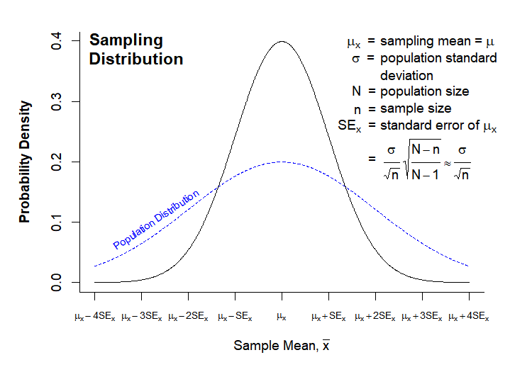
The figure contrasts the wider population distribution with the narrower sampling distribution of the sample mean, highlighting that standard error represents the spread of the sampling distribution. As sample size increases or the sampling fraction remains small, the sampling distribution tightens. The inclusion of the finite population correction aligns with the 10% condition discussed in the notes. Source.
This formula highlights two key ideas:
• Increasing sample size reduces variability.
• Populations with greater inherent variability contribute more to the overall spread.
The standard deviation of a sampling distribution is commonly called the standard error, though this subsubtopic focuses on the theoretical form based on known population parameters.
Finite Population Considerations
In many practical settings, sampling is conducted without replacement, meaning sampled individuals are not returned to the population before drawing the next. This situation creates slight dependence between selections, which normally requires a finite population correction (FPC) to adjust the standard deviation.
However, when the sample size is less than 10% of the population, the difference between sampling with and without replacement becomes negligible. Therefore, AP Statistics permits omitting the correction under this condition. This simplification maintains conceptual clarity while remaining mathematically sound.
Conditions Supporting Parameter Determination
To confidently apply these formulas, several conditions must hold:
Independence of Samples
• The two populations must not influence each other.
• Random sampling or random assignment helps uphold independence.
• Independence ensures that combining variances is appropriate and does not introduce bias into the sampling distribution.
Known or Assumed Population Parameters
• The formulas rely on knowing or reasonably estimating σ₁ and σ₂.
• In practice, these may be estimated from data, but the theoretical structure assumes known values to define the sampling distribution.
Correct Sample Size Interpretation
• Larger sample sizes shrink the standard deviation of the sampling distribution.
• Differences in sample sizes between the two samples influence how each population contributes to overall sampling variability.
Why These Parameters Matter
Understanding the parameters of the sampling distribution for differences in sample means is essential for inference because they allow researchers to:
• Assess how much observed differences could be due to random sampling variation.
• Construct probability statements about the difference between population means.
• Prepare for future topics such as confidence intervals and significance testing for comparing means.
FAQ
Increasing just one sample size reduces the contribution of that population’s variability to the overall standard deviation, making the sampling distribution narrower.
The reduction is not symmetrical:
• Increasing the sample size for the population with the larger standard deviation tends to have a greater effect.
• If one sample size remains very small, it can dominate the total variability even if the other is large.
Independence ensures that variation in one sample does not influence the other, allowing variances to add directly.
If the samples were dependent, the covariance between the sample means would alter the spread of the distribution. This could either increase or decrease variability, depending on the relationship, making the standard formula invalid.
The shape of the sampling distribution still depends on the behaviour of the sample means, not the populations themselves.
If sample sizes are sufficiently large, the Central Limit Theorem ensures that each sample mean is approximately normal, so their difference is also approximately normal.
If either sample size is small, skewed or heavy-tailed population shapes can make the resulting distribution noticeably non-normal.
Treating the expression as a single statistic allows clearer interpretation and simpler inference because it captures the contrast of interest directly.
It also permits:
• A single mean (the difference in population means).
• A single measure of variability (the combined variance).
• A straightforward approach for confidence intervals and hypothesis tests targeting the difference.
Small inaccuracies in population standard deviations generally produce modest changes in the combined standard deviation.
The effect is larger when:
• The misestimated population has a high true variability.
• The sample size for that population is small, giving its variance term greater weight.
In applied settings, using sample-based estimates introduces additional uncertainty, but the structure of the formula still provides a robust approximation.
Practice Questions
Question 1 (1–3 marks)
A researcher takes two independent random samples, one from Population A and one from Population B. The population standard deviation of A is known to be 12, and that of B is 16. The researcher plans to take a sample of size 36 from each population.
(a) State the mean of the sampling distribution of the difference in sample means (A minus B).
(b) Calculate the standard deviation of the sampling distribution of the difference in sample means.
Question 1
(a) 1 mark
• States that the mean of the sampling distribution equals the difference in population means (A minus B).
• Award the mark even if the numerical value is not given (since population means are not provided).
(b) 2 marks
• 1 mark for correctly identifying the formula: sqrt( (12^2 / 36) + (16^2 / 36) ).
• 1 mark for correct simplification to the final value: sqrt(4 + 7.11...) ≈ 3.35.
(Allow minor rounding differences.)
Total: 3 marks
Question 2 (4–6 marks)
A nutritionist is comparing the average sugar content in two brands of fruit yoghurt, Brand X and Brand Y. The population standard deviations are known: 5 grams for Brand X and 7 grams for Brand Y. Independent random samples of size 25 are taken from each brand, with sample means of 18.2 grams (X) and 20.0 grams (Y).
(a) Explain why the sampling distribution of the difference in sample means can be modelled using the standard formula for its mean and standard deviation.
(b) Determine the mean of the sampling distribution of (X minus Y).
(c) Compute the standard deviation of the sampling distribution of (X minus Y).
(d) Briefly comment on what the magnitude of the standard deviation implies about the variability of the statistic in repeated sampling.
Question 2
(a) 2 marks
• 1 mark for stating that the samples are independent.
• 1 mark for recognising that population standard deviations are known and sample sizes are sufficiently large for the formula to hold.
(b) 1 mark
• Gives the mean of the sampling distribution: 18.2 − 20.0 = −1.8 grams.
(c) 2 marks
• 1 mark for stating or using the correct formula: sqrt( (5^2 / 25) + (7^2 / 25) ).
• 1 mark for correct computation: sqrt(1 + 1.96) ≈ 1.67 grams.
(d) 1 mark
• Provides a sensible interpretation: for example, that a standard deviation of about 1.67 grams indicates moderate variability in the difference of sample means across repeated samples.
Total: 6 marks
