
AQA Specification focus:
‘The difference between fixed and variable costs; the difference between marginal, average and total costs; the difference between short-run and long-run costs; the reasons for the shape of the marginal, average and total cost curves.’
Introduction
Understanding costs of production is fundamental in A-Level Economics, as it explains how firms make decisions regarding output and pricing. Costs shape supply behaviour, profitability, and industry structure.
Types of Cost
Fixed and Variable Costs
Costs are categorised into fixed and variable in the short run.
Fixed Costs: Costs that do not vary with the level of output, such as rent, insurance, or salaries of permanent staff.
These remain constant regardless of production volume in the short run.
Variable Costs: Costs that change with the level of output, such as raw materials, energy usage, or wages of temporary workers.
Firms face both types of costs simultaneously. In the long run, however, all costs become variable because firms can adjust all factor inputs.
Total, Average and Marginal Costs
Firms must also distinguish between different cost measures to make efficient production decisions.
Total Cost (TC): The sum of fixed and variable costs at each level of output.
Average Cost (AC): Total cost divided by the quantity of output produced (AC = TC ÷ Q).
This is also referred to as unit cost.
Marginal Cost (MC): The additional cost of producing one extra unit of output.
These three measures are interrelated and are represented on standard cost curves.
Short Run vs Long Run Costs
The Short Run
In the short run, at least one factor of production is fixed. Firms can adjust output only by varying variable inputs, like labour or raw materials. Consequently:
Fixed costs remain constant, regardless of output.
Variable costs rise with increased output.
Total costs are the sum of both.
This leads to characteristic cost curve shapes, especially for marginal cost and average cost.
The Long Run
In the long run, all factors of production are variable. Firms can expand capacity, purchase new machinery, or move premises. This flexibility allows them to exploit economies of scale, reducing average costs as output grows. Long-run cost curves therefore differ in shape from short-run ones.
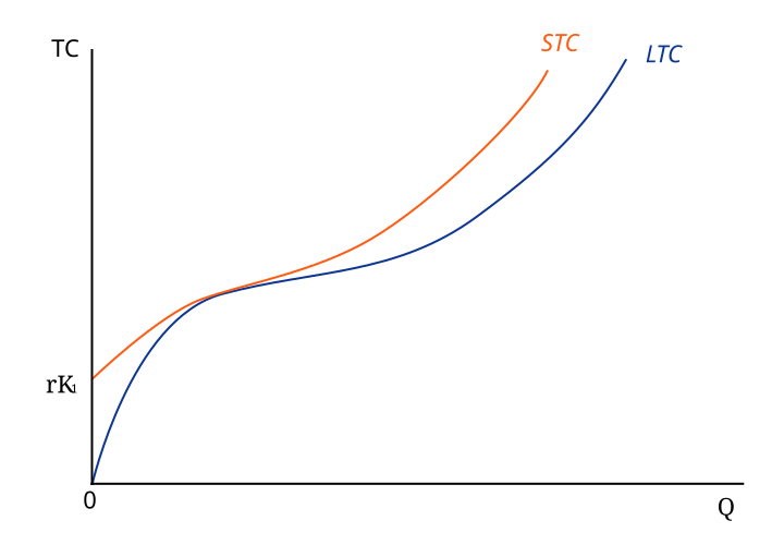
This diagram shows the relationship between short-run cost curves (SRAC) and the long-run cost curve (LRAC). It demonstrates how firms can adjust all factors of production in the long run, leading to potential economies of scale and a flatter LRAC curve. Source
Cost Curve Shapes
Marginal Cost Curve
The MC curve typically falls at first due to increasing returns from variable inputs, but eventually rises because of the law of diminishing returns.
Initially, adding more workers can increase productivity, lowering the cost of producing each extra unit.
Beyond a certain point, overcrowding or inefficiency causes marginal cost to rise.
This U-shape is fundamental in microeconomics.
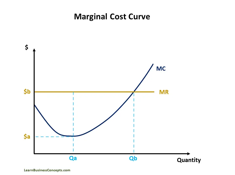
The marginal cost (MC) curve typically exhibits a U-shape, initially decreasing as production increases due to increasing returns, and then rising as diminishing returns set in. This shape reflects the changing cost of producing additional units. Source
Average Cost Curve
The AC curve is also typically U-shaped in the short run:
Falling at first as fixed costs are spread over more units of output.
Rising later when diminishing returns push variable costs upward.
Importantly, the AC curve always intersects with the MC curve at the AC’s minimum point. This relationship is mathematically necessary.
Total Cost Curve
The TC curve starts at the level of fixed costs when output is zero and rises as output increases. Its slope at any given point represents marginal cost.
Relationship Between Costs
Links Between Marginal and Average Costs
When MC < AC, average cost falls.
When MC > AC, average cost rises.
When MC = AC, average cost is at its minimum.
This relationship helps explain why the MC curve cuts the AC curve at the lowest point of the AC.
Short Run vs Long Run Curve Shapes
In the short run, cost curves are U-shaped due to diminishing returns.
In the long run, the average cost curve reflects economies and diseconomies of scale. This gives the curve a broader U-shape, sometimes depicted as L-shaped to reflect persistent efficiency gains at higher output.
Equations for Costs
Total Cost (TC) = Fixed Cost (FC) + Variable Cost (VC)
TC = Combined cost of production at any output level
Average Cost (AC) = Total Cost ÷ Quantity (Q)
AC = Cost per unit of output
Marginal Cost (MC) = ΔTotal Cost ÷ ΔQuantity
MC = Additional cost from producing one extra unit
These formulae are central for interpreting data and constructing cost curves.
Reasons for Cost Curve Shapes
Short Run
Fixed cost spreading: Average fixed cost falls as output increases, pulling down average cost.
Law of diminishing returns: As variable inputs increase, marginal productivity eventually declines, raising marginal and average costs.
Long Run
Economies of scale: Larger output allows cost savings, e.g. through bulk purchasing or specialisation.
Diseconomies of scale: Very large scale may cause rising costs due to management difficulties or communication breakdowns.
Together, these factors shape the long-run average cost curve (LRAC). It declines at first, flattens, and may eventually rise.
Practice Questions
Define the terms fixed cost and marginal cost, and briefly state one difference between them. (3 marks)
1 mark for a correct definition of fixed cost: costs that do not vary with the level of output (e.g. rent, insurance).
1 mark for a correct definition of marginal cost: the additional cost of producing one more unit of output.
1 mark for a clear difference identified (e.g. fixed costs remain constant regardless of output, whereas marginal cost depends on changes in variable costs/output).
Explain, with the use of a diagram, why the average cost (AC) curve is typically U-shaped in the short run. (6 marks)
1 mark for correctly identifying that average costs fall initially due to the spreading of fixed costs.
1 mark for explaining that increasing returns to variable inputs also reduce costs at lower output levels.
1–2 marks for explaining that average costs rise at higher output levels due to diminishing returns.
1–2 marks for a correctly drawn and clearly labelled U-shaped AC curve diagram.
Maximum of 6 marks available.
FAQ
Fixed costs exist in the short run because certain inputs, like premises or machinery, cannot be changed immediately. Firms must continue paying these costs regardless of output.
In the long run, all costs are variable because firms have time to change all factor inputs, such as relocating, upgrading machinery, or renegotiating contracts. This flexibility removes the concept of fixed costs.
Sunk costs are fixed costs that cannot be recovered once spent, even if production stops. Examples include advertising campaigns or research and development expenses.
Not all fixed costs are sunk costs; rent is fixed but may be avoided if a lease ends. The key distinction lies in whether the cost is recoverable.
The marginal cost (MC) curve helps firms decide the profit-maximising output. Profit maximisation occurs when MC = MR (marginal revenue).
It also signals efficiency. If marginal cost is below average cost, producing more lowers average costs. If above, producing more raises them. This makes the MC curve central to pricing and output strategies.
Several factors can alter the AC curve’s shape:
Fixed cost distribution: Lower average fixed costs as output increases.
Productivity changes: Improvements in labour efficiency can shift the curve downward.
Input prices: Rising wages or raw material prices steepen the upward slope.
These influences explain why AC curves vary across industries.
Yes, in rare cases where firms benefit from sustained economies of scale without significant diseconomies.
Examples include digital products, where once initial development costs are covered, the marginal and average costs of producing extra copies approach zero.
In such cases, the AC curve can resemble an L-shape rather than the typical U-shape.
