

Question 1
Students investigated a hypothetical non-mobile plant population in a meadow. Random quadrats were placed at sites with different soil pH values, and plant density was recorded. Other environmental variables were not controlled.
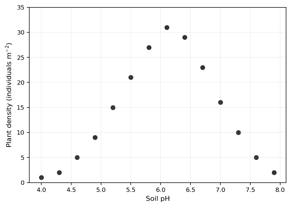
Describe the relationship between soil pH and plant density shown in the graph.
Estimate the soil pH at which the greatest plant density occurs and identify an approximate pH range in which density remains relatively high.
Analyse the extent to which the graph supports the conclusion that soil pH determines the distribution of this plant population.
Question 2
A hypothetical population was monitored for months in an ecosystem with no major external disturbance.
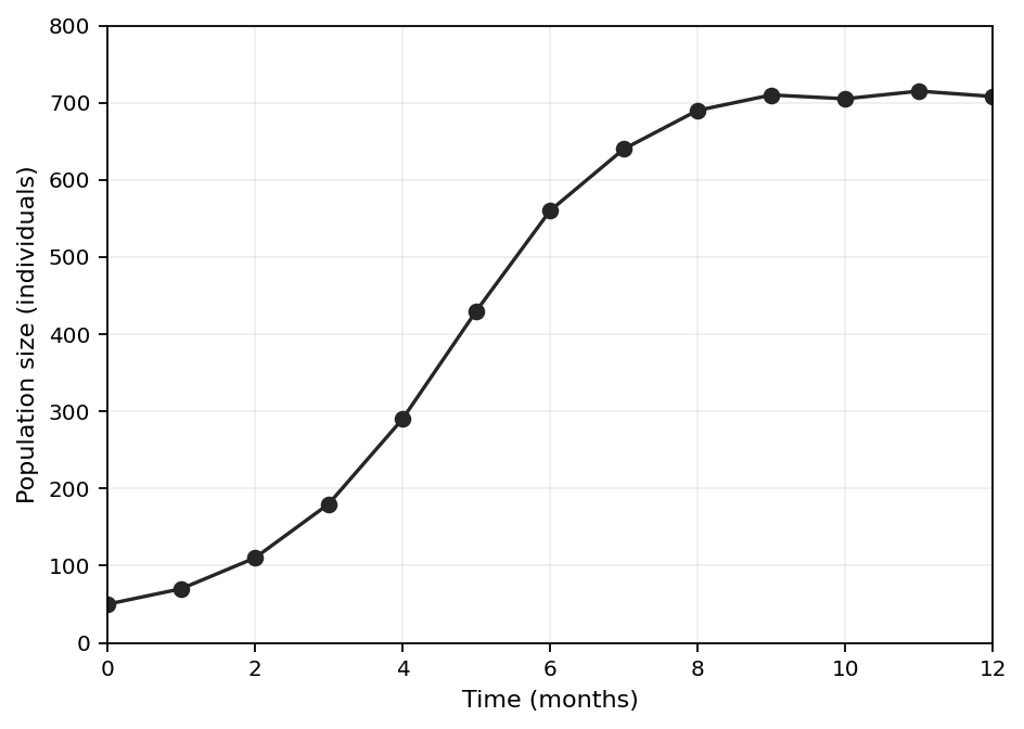
Estimate the carrying capacity indicated by the graph.
Compare the rate of population growth between months – and months –.
Explain how density-dependent factors and negative feedback could produce the pattern observed after month .
Predict the likely population response if population size temporarily increased substantially above the carrying capacity, assuming environmental conditions remained similar.
Question 3
The graph shows synthetic monitoring data for interacting predator and prey populations in a hypothetical ecosystem.
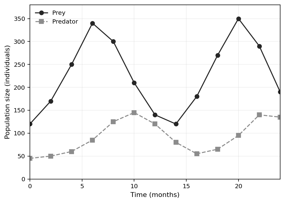
Describe two features of the relationship between predator and prey population size.
Using the first major population peaks, estimate the time lag between the prey peak and predator peak.
Explain how predation can produce the repeated population changes shown.
Question 4
A student is investigating the abundance of a non-mobile plant species in a terrestrial ecosystem. The photograph below shows a quadrat that could be placed at sampling locations across the study area.
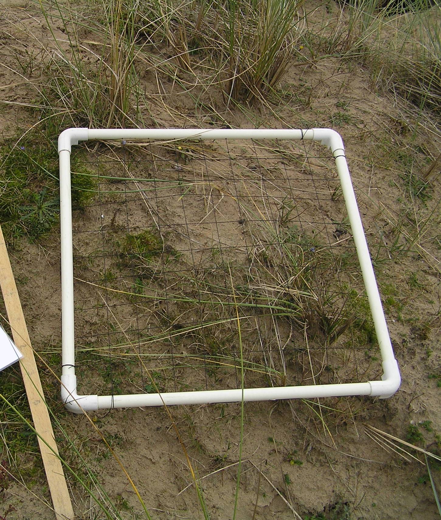
Identify two visible features of the sampling device that make it suitable for estimating percentage cover.
Explain how random quadrat sampling could be used to estimate the abundance of the plant species across the larger study area.
Evaluate the reliability of using only the single quadrat placement shown in the photograph, and suggest one improvement.
Question 5
The diagram below represents feeding relationships in a forest ecosystem. The legend shows that arrows point from what is eaten towards what eats it. Organisms are also arranged into broad trophic categories. Species identification is not required; organisms may be described by their appearance or position.
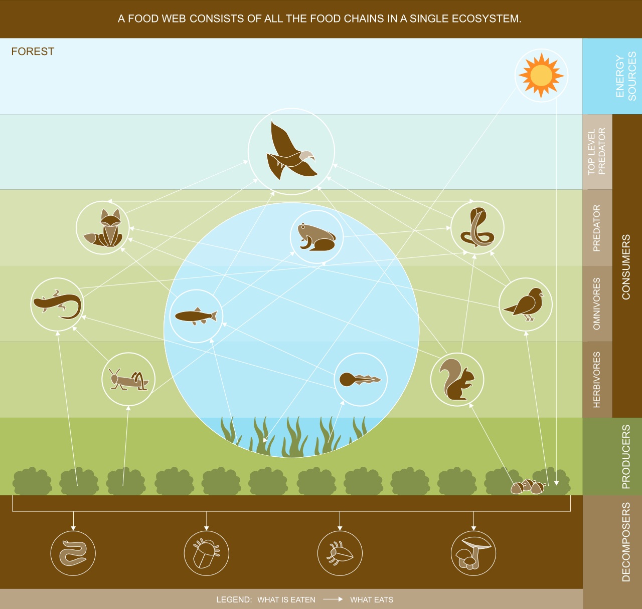
Using the direction of the arrows, outline one feeding pathway shown that contains at least three trophic levels.
Analyse how the pattern of cross-linked arrows in the diagram demonstrates why a food web represents trophic relationships more completely than a single food chain.
Predict the effect of a sustained reduction in producer biomass on one higher-level consumer shown in the diagram. Explain your prediction.
Question 6
The ecological pyramid below represents the relative quantity of food energy associated with successive trophic levels in an ecosystem. Interpret the relative sizes of the tiers qualitatively rather than attempting to obtain numerical values.
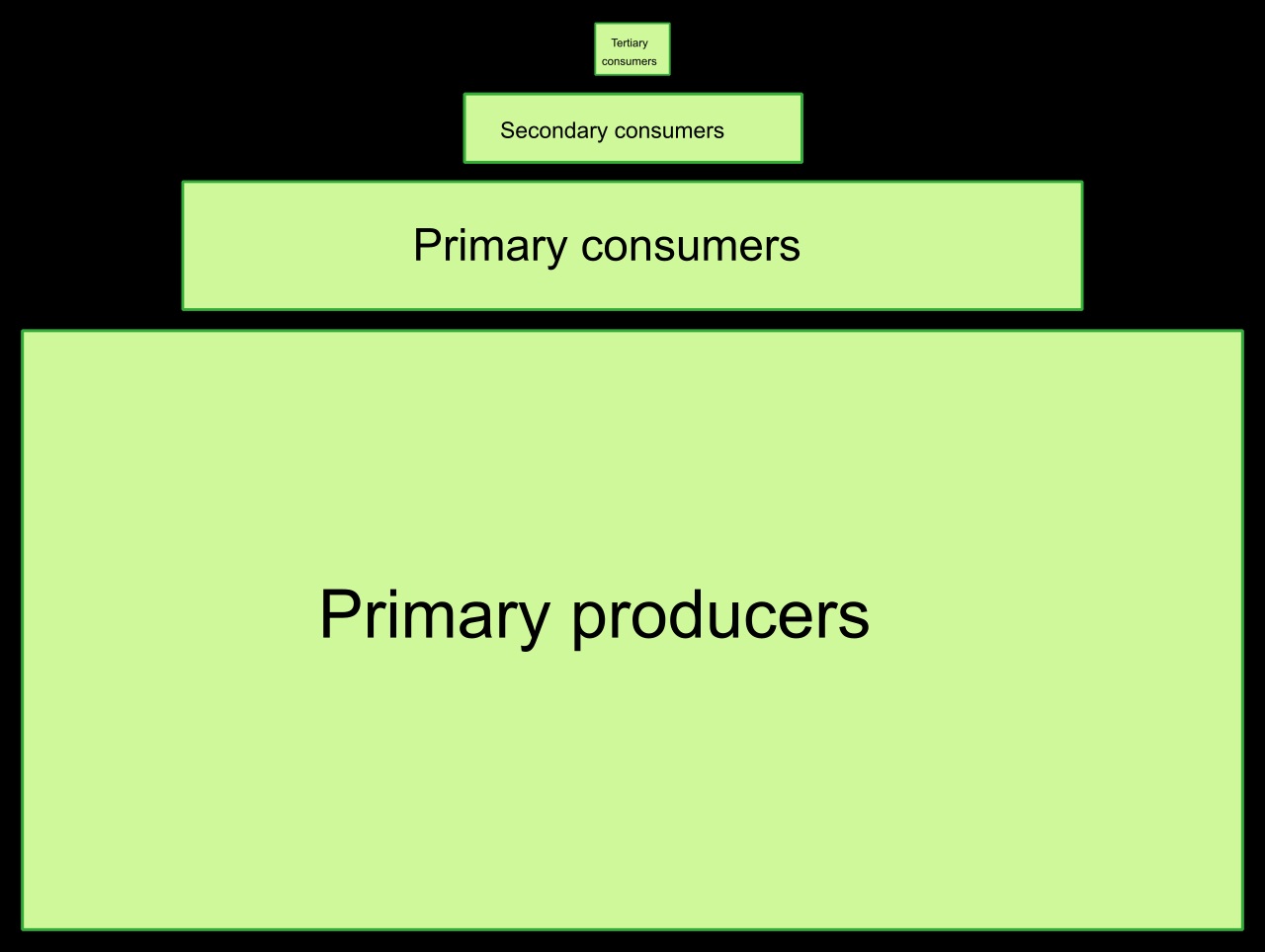
Describe the pattern in tier size from primary producers to tertiary consumers.
Explain why the energy pattern visible in the pyramid occurs as food passes from one trophic level to the next.
Explain how the pattern shown helps account for the limited number of trophic levels in most ecosystems.
Question 7
The diagram below represents the carbon cycle and shows several carbon stores and flows. Arrows link the atmosphere, vegetation, soil, oceans, marine organisms and sediments, while human fossil-fuel emissions are also shown.
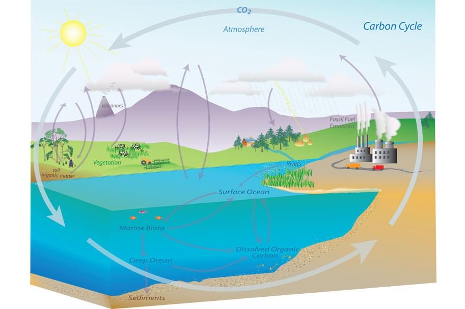
Identify two carbon stores visible in the diagram.
Using two arrows visible between the atmosphere and either vegetation or the ocean, explain the processes responsible for the carbon flows represented.
Fossil-fuel emissions are shown as a flow into the atmosphere. Explain why an increase in this flow can cause atmospheric carbon dioxide to accumulate even though ecosystems and oceans can act as carbon sinks.
Question 8
The sequence below shows the same shell during a laboratory experiment. It was exposed for 45 days to seawater adjusted to ocean-chemistry conditions projected for 2100.
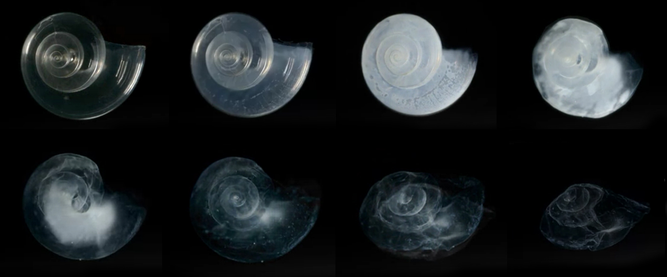
Describe two visible changes in the shell across the sequence.
Explain how an increase in dissolved carbon dioxide in seawater could produce the changes visible in the sequence.
Predict one effect on a marine food web if populations of shell-forming organisms affected in this way were substantially reduced. Explain your answer.
Question 9
The diagram below represents global atmospheric circulation. The equator and latitudes of approximately and north and south are marked, together with major surface winds and circulation loops.
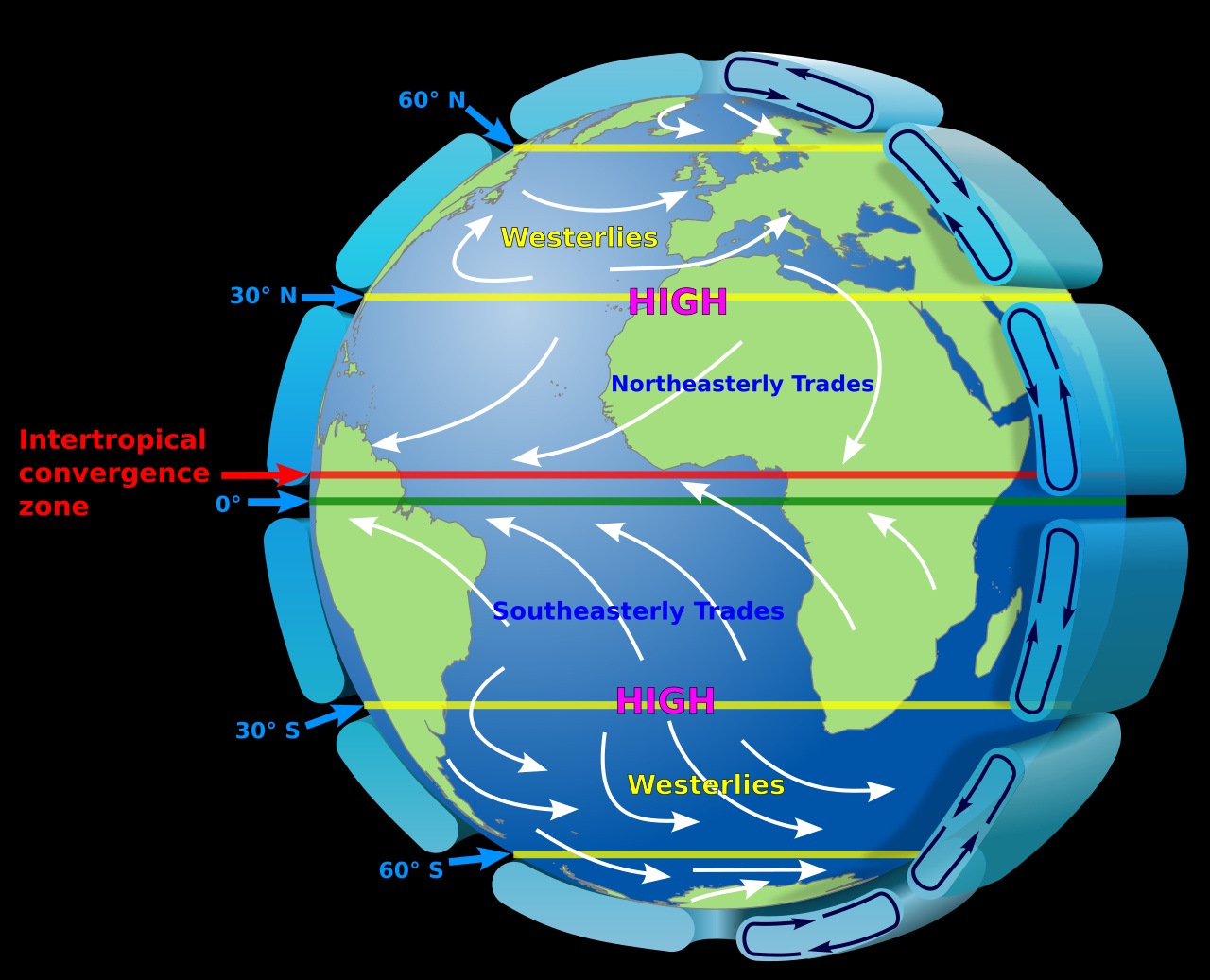
Identify the atmospheric circulation cell operating mainly between the equator and approximately latitude, and state the pressure condition marked near .
Using the circulation pattern shown, explain why precipitation is generally greater close to the equator than around latitude.
Explain how this atmospheric pattern contributes to the broad distribution of tropical rainforest and hot desert biomes.
Question 10
The photograph below shows researchers using quadrats and a transect arrangement on an intertidal shore. Such sampling can be used to investigate changes in a community along an environmental gradient.
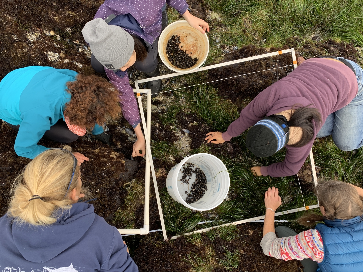
Identify two visible features of the sampling arrangement that could be used to collect data systematically along an environmental gradient.
Explain why placing quadrats along a transect is appropriate for investigating zonation.
Suggest two abiotic factors that could be measured at locations along this transect and explain how variation in each could help account for differences in species distribution.