Analysing experimental data in A-Level Physics requires applying mathematical skills accurately to identify relationships, test predictions, and quantify physical principles. Mastery of these skills ensures data is interpreted correctly and scientific conclusions are valid.

Core Mathematical Applications in Physics

Mathematical analysis transforms raw experimental data into meaningful physical relationships. It allows students to move from observation to quantitative understanding, testing theoretical models against measured evidence.

Key Mathematical Skills

OCR expects candidates to:

• Use algebraic manipulation to rearrange equations.

• Apply ratios, fractions, and percentages in data interpretation.

• Employ standard form, prefixes, and unit conversions correctly.

• Calculate and interpret gradients and intercepts from graphs.

• Analyse proportional relationships between variables.

• Perform statistical analysis for evaluating data reliability.

Algebraic Manipulation and Rearrangement

Most physical relationships involve equations connecting multiple variables. Accurate rearrangement ensures correct substitution and computation.

Common operations include:

• Rearranging equations to isolate a specific variable.

• Combining or substituting equations to eliminate unknowns.

• Checking dimensional consistency after rearrangement.

EQUATION
—-----------------------------------------------------------------
Ohm’s Law (V) = I × R
V = Potential difference (volt, V)
I = Current (ampere, A)
R = Resistance (ohm, Ω)
—-----------------------------------------------------------------

Rearranging this equation, for example, enables the calculation of current from known voltage and resistance values. This reinforces the importance of algebraic fluency in experimental work.

Ratios, Proportions, and Percentage Change

Physics often explores how one quantity changes relative to another. Recognising proportionality is vital for deducing underlying laws.

These skills are used when analysing data such as current–voltage graphs or temperature–resistance trends.

Students should be able to:

• Express proportional relationships as equations, e.g. y = kx.

• Identify inverse and square relationships, e.g. y ∝ 1/x or y ∝ x².

• Calculate percentage change to compare data points or assess accuracy.

EQUATION
—-----------------------------------------------------------------
Percentage Change (%) = (Change / Original Value) × 100
Change = Difference between two measured or calculated quantities
Original Value = Baseline measurement or theoretical value
—-----------------------------------------------------------------

This allows comparisons across trials and assessment of trends.

Handling Units and Prefixes

Correct unit usage is a foundation of reliable analysis. Every derived quantity must be expressed in SI units to maintain consistency.

Common SI Prefixes

• milli (m) = 10⁻³

• micro (µ) = 10⁻⁶

• kilo (k) = 10³

• mega (M) = 10⁶

Students must convert units consistently before performing calculations or plotting graphs. For example, converting milliamperes to amperes or centimetres to metres avoids scaling errors in derived values.

Graphical Analysis of Quantitative Data

Graphs reveal patterns and relationships hidden within numerical data, serving as a powerful tool for interpreting results.

Constructing Graphs

When plotting data:

• Place the independent variable on the x-axis and dependent variable on the y-axis.

• Label both axes with quantities and units.

• Use scales that allow easy reading and minimise uncertainty.

• Include error bars where appropriate.

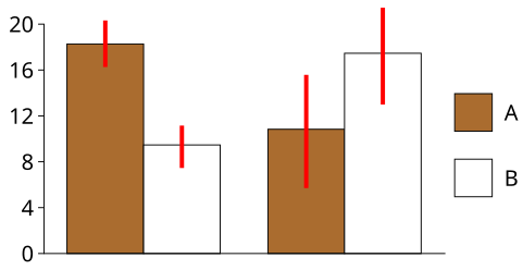
A column chart with red vertical confidence-interval bars showing how uncertainty is represented around point estimates. Such bars can indicate standard deviation, standard error, or confidence intervals, illustrating how data reliability is visualised in physics graphs. Source

Interpreting Graphs

• Identify linear relationships and determine the gradient.

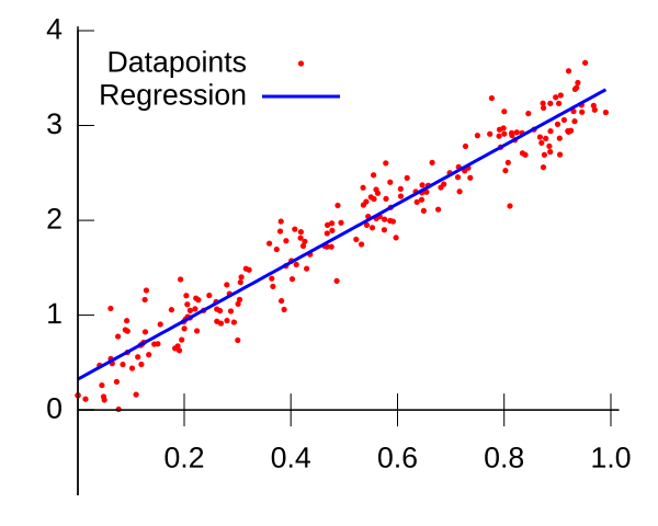
A scatter plot with a straight regression line illustrating how experimental data are modelled linearly. The gradient represents the physical constant derived from the relationship, while the intercept shows any fixed offset. Both axes are labelled clearly to highlight correct unit usage. Source

• Use the intercept to infer constants or offsets in equations.

• Apply line of best fit to estimate underlying relationships.

EQUATION
—-----------------------------------------------------------------
Gradient (m) = Δy / Δx
Δy = Change in the dependent variable (unit depends on variable)
Δx = Change in the independent variable (unit depends on variable)
—-----------------------------------------------------------------

Gradients are crucial for deriving quantities such as resistance, spring constant, or acceleration.

Use of Logarithmic and Power Relationships

Some data produce non-linear graphs. By taking logarithms, these can often be linearised for easier analysis.

For instance, if y ∝ xⁿ, then plotting log(y) against log(x) gives a straight line with gradient n.

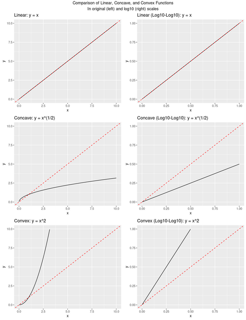
A comparison of graphs plotted on original and log–log scales. On log–log axes, power-law relationships appear as straight lines whose gradient equals the exponent, demonstrating the process of linearising non-linear data in experimental analysis. Source

Recognising and applying these transformations demonstrates deeper understanding of physical laws.

Statistical Treatment of Data

Statistical methods enhance confidence in experimental results by quantifying variability and uncertainty.

Mean and Range

Calculating the mean of repeated measurements reduces random error, while the range indicates the spread of data.

EQUATION
—-----------------------------------------------------------------
Mean (x̄) = Σx / n
Σx = Sum of all measurements (unit depends on quantity)
n = Number of measurements
—-----------------------------------------------------------------

Students should also understand the standard deviation as a measure of data spread around the mean.

Evaluating Reliability

• Identify outliers that deviate significantly from the mean.

• Use error bars to represent uncertainty visually.

• Compare overlapping error ranges to assess significance of differences.

Mathematical Modelling and Linearisation

Physical data often follow models that can be simplified through linear equations for ease of analysis.

Linearisation Process

1. Start from a known physical relationship (e.g. Hooke’s law, Boyle’s law).

2. Rearrange the formula to match y = mx + c form.

3. Plot appropriate variables to yield a straight-line graph.

4. Interpret gradient and intercept in terms of physical constants.

Understanding how to linearise data ensures accurate determination of constants such as resistivity or spring stiffness.

Dimensional Analysis

Dimensional analysis acts as a consistency check, confirming whether an equation or rearrangement is physically valid.

EQUATION
—-----------------------------------------------------------------
Dimensional Consistency: [Quantity] = [Base Units]
Example: Force = mass × acceleration
F = kg × m s⁻² = kg·m·s⁻²
—-----------------------------------------------------------------

If dimensions on both sides of an equation match, the expression is likely correct, though not guaranteed numerically accurate.

Use of Ratios and Proportional Reasoning in Experiments

When analysing experimental outcomes, proportional reasoning provides insight into how changing one variable influences another. This is particularly important when direct measurement is difficult.

Students must:

• Recognise direct, inverse, and square proportionalities.

• Calculate ratios to compare multiple experiments.

• Use normalised data to remove dependency on absolute magnitudes.

Final Emphasis on Mathematical Precision

Applying mathematical skills correctly ensures that physical interpretations are quantitatively justified. The OCR specification emphasises precise manipulation of numbers, equations, and data presentation as core competencies for all experimental and analytical work. Mastery of these mathematical foundations enables the clear, confident evaluation of physical systems and reliable evidence-based conclusions.