
OCR Specification focus:
‘Discuss precision and accuracy, calculate margins of error and percentage errors, and account for uncertainties in apparatus and measurements.’
Precision, accuracy, and uncertainties are essential aspects of experimental physics, ensuring that data are reliable, comparable, and scientifically valid. Understanding these concepts helps evaluate experimental quality and interpret results meaningfully.
Understanding Precision and Accuracy
Precision
Precision refers to the repeatability and consistency of measurements. When repeated measurements yield values close to each other, the data set is considered precise, even if the results are not necessarily accurate. Precision depends on random errors, which affect how spread out repeated readings are.
Precision: The degree to which repeated measurements under unchanged conditions show the same results.
High precision implies small random uncertainty, often assessed through the range or standard deviation of results.
Accuracy
Accuracy measures how close a result is to the true or accepted value. A measurement can be precise without being accurate if it consistently deviates due to systematic error. Accuracy depends on eliminating or minimising systematic errors from instruments, calibration, or environmental factors.
Accuracy: The closeness of a measured or derived value to the true or accepted value of the quantity.
Relationship between Precision and Accuracy
Both are vital for experimental validity.
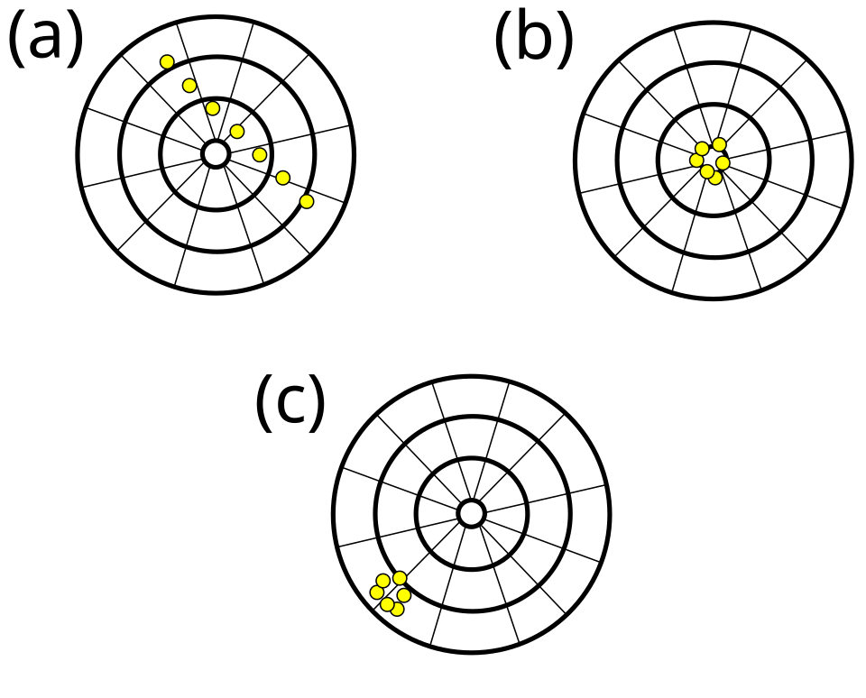
This bullseye graphic contrasts accuracy and precision: tightly clustered hits show precision, while proximity to the centre shows accuracy. A result can be precise yet inaccurate, accurate yet imprecise, or both. The diagram aligns with the definitions used when evaluating experimental data quality. Source.
A measurement system can be:
Accurate but imprecise – results close to the true value but with wide scatter.
Precise but inaccurate – clustered results far from the true value.
Accurate and precise – ideal case, consistent and close to the accepted value.
In all experiments, the goal is to maximise both precision and accuracy through careful technique, calibration, and data handling.
Understanding Uncertainties
Types of Uncertainty
Uncertainties describe the limits within which the true value is expected to lie. No measurement is exact; every reading carries an inherent level of doubt. Uncertainties can be classified as:
Random uncertainties: arise from unpredictable variations in conditions or human judgement (e.g., reading fluctuations on an analogue scale).
Systematic uncertainties: occur due to consistent bias in measurements, such as miscalibrated instruments or zero errors.
Estimating Uncertainties in Measurements
To account for uncertainty, physicists estimate a range around a measurement. Typical rules include:
For analogue instruments, uncertainty is ± half the smallest division.
For digital instruments, uncertainty is ± the smallest displayed unit.
For multiple readings, the uncertainty in the mean can be estimated as half the range or standard deviation divided by √n, depending on context.
EQUATION
—-----------------------------------------------------------------
Uncertainty in mean (Δx) = Range ÷ 2 or Standard deviation ÷ √n
Δx = Estimated uncertainty in mean (same units as x)
n = Number of measurements (no unit)
—-----------------------------------------------------------------
Understanding these conventions ensures consistency across practical investigations.
Percentage Uncertainty
Percentage uncertainty allows comparison of reliability between different quantities or instruments. It expresses uncertainty as a fraction of the measured value, multiplied by 100.
EQUATION
—-----------------------------------------------------------------
Percentage uncertainty = (Absolute uncertainty ÷ Measured value) × 100
Absolute uncertainty = Measurement uncertainty (same units as measured value)
Measured value = Quantity being measured (any appropriate unit)
—-----------------------------------------------------------------
The smaller the percentage uncertainty, the more reliable the measurement.
Combining Uncertainties
In experiments involving multiple quantities, uncertainties combine depending on the mathematical operation:
Addition or subtraction: add absolute uncertainties.
Multiplication or division: add percentage uncertainties.
Powers or roots: multiply the percentage uncertainty by the power value.
These rules ensure that uncertainties are propagated logically through derived quantities such as area, volume, or calculated constants.
EQUATION
—-----------------------------------------------------------------
For a quantity Z = A × B or Z = A ÷ B,
Percentage uncertainty in Z = (Percentage uncertainty in A + Percentage uncertainty in B)
A, B, Z = Physical quantities with appropriate units
—-----------------------------------------------------------------
Consistent application of these rules ensures valid comparison and evaluation of experimental data.
Margins of Error and Error Calculations
Margin of Error
The margin of error indicates the range around a measurement that likely contains the true value. It provides context for uncertainty when quoting results.
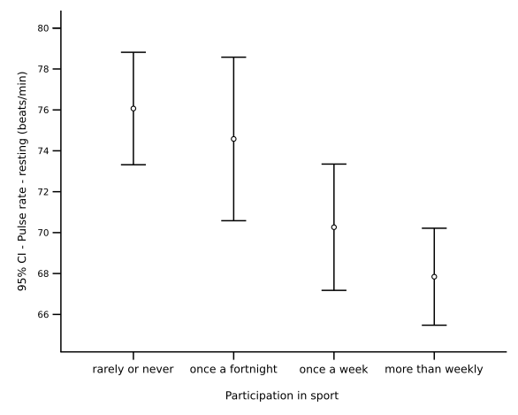
The chart shows mean values with 95% confidence-interval error bars, illustrating how uncertainty is displayed graphically. Shorter bars indicate more precise estimates; wider bars indicate greater variability or uncertainty. This aligns with expressing results as a value ± uncertainty. Source.
For example, reporting a length as 20.0 ± 0.5 cm communicates both the measured value and its uncertainty range. The result should always include the uncertainty to the same decimal place as the measurement.
Percentage Error
Percentage error compares an experimental result with an accepted or theoretical value. It provides insight into how accurate an experiment was.
EQUATION
—-----------------------------------------------------------------
Percentage error = (|Experimental value – True value| ÷ True value) × 100
Experimental value = Obtained measurement (any unit)
True value = Accepted theoretical or reference value (same unit)
—-----------------------------------------------------------------
A small percentage error suggests high accuracy; however, even small systematic errors can lead to significant inaccuracies if unaccounted for.
Reducing Uncertainty and Improving Reliability
To improve experimental reliability and minimise uncertainty:
Increase the number of readings and calculate an average to reduce random effects.
Use instruments with smaller scale divisions or higher resolution for greater precision.
Calibrate equipment regularly to avoid systematic bias.
Control environmental variables, such as temperature or vibration, that may introduce random fluctuations.
Avoid parallax error by reading analogue scales at eye level.
Repeat experiments to confirm reproducibility and detect anomalies.
By applying these strategies, students ensure data are scientifically credible and reproducible, aligning with the OCR expectation of evaluating experimental quality using precision, accuracy, and uncertainty principles.
Practice Questions
Question 1 (2 marks)
A student measures the diameter of a wire using a micrometer screw gauge. The readings are:
Trial 1: 0.52 mm Trial 2: 0.50 mm Trial 3: 0.51 mm
(a) Calculate the mean diameter of the wire.
(b) State the uncertainty in the mean diameter.
Mark scheme for Question 1
(a) Correct mean calculation: (0.52 + 0.50 + 0.51) ÷ 3 = 0.51 mm (1 mark)
(b) Correct estimation of uncertainty: ±0.01 mm (half the range = 0.02 ÷ 2) (1 mark)
Award full marks only if both the mean and uncertainty include correct units and appropriate significant figures.
Question 2 (5 marks)
An experiment is carried out to determine the acceleration due to gravity, g, by timing the fall of a small ball bearing. The measured fall distance is 1.20 m ± 0.01 m and the average time of fall is 0.495 s ± 0.005 s.
(a) Use the equation g = 2s / t² to calculate the value of g.
(b) Calculate the percentage uncertainty in g.
(c) Discuss one way to reduce the uncertainty in this experiment.
Mark scheme for Question 2
(a) Substitution and calculation:
g = 2 × 1.20 ÷ (0.495)² = 9.8 m s⁻² (accept 9.7–9.9) (1 mark)
(b) Correct percentage uncertainty method:
For g = 2s / t², combine uncertainties:
Percentage uncertainty in g = (percentage uncertainty in s) + (2 × percentage uncertainty in t) (1 mark)
Percentage uncertainty in s = (0.01 ÷ 1.20) × 100 = 0.83% (1 mark)
Percentage uncertainty in t = (0.005 ÷ 0.495) × 100 = 1.0% (1 mark)
Total = 0.83% + 2.0% = 2.8% (1 mark)
(c) Sensible suggestion with justification: e.g.
Use a light gate instead of manual timing to reduce reaction time errors (1 mark)
Or increase drop height to make timing uncertainty smaller relative to total time (1 mark)
(Maximum 5 marks total)
FAQ
Random uncertainty arises from small, unpredictable fluctuations in experimental conditions or instrument behaviour, such as vibration or temperature drift. It affects the precision of results.
Human error, however, refers to mistakes made during measurement or recording — for example, misreading a scale or forgetting to zero an instrument. These are not part of the inherent uncertainty and should be avoided through careful technique, whereas random uncertainty is unavoidable but can be reduced by repeating measurements.
Calibration aligns an instrument’s readings with a known standard, ensuring that systematic errors are minimised.
If an instrument consistently gives readings higher or lower than the true value, calibration allows you to apply a correction.
Regular calibration ensures accuracy across multiple experiments, especially for sensors and digital apparatus where drift can occur over time.
This process improves confidence that measured values represent true physical quantities.
Consistency of decimal places ensures numerical coherence and avoids implying false precision.
If a length is measured as 1.23 m with an uncertainty of ±0.004 m, the uncertainty should be rounded to ±0.01 m and reported as 1.23 ± 0.01 m.
Quoting mismatched precision (e.g. 1.234 ± 0.1) suggests an inaccurate understanding of measurement reliability, undermining the credibility of reported data.
Repeating a measurement reduces random uncertainty because averaging multiple results cancels out unpredictable variations.
However, systematic uncertainties remain unaffected — for example, a miscalibrated sensor will produce the same bias each time.
To improve overall reliability:
Repeat readings to reduce random effects.
Recalibrate or change equipment to address systematic effects.
This dual approach ensures both precision and accuracy are improved.
Error bars visually represent uncertainty on a graph, showing the potential range of the true value. They make data reliability immediately visible.
Uncertainty in tabulated data is the same concept but expressed numerically, often written as a value ± uncertainty.
Error bars are particularly useful when comparing datasets: overlapping bars imply differences may not be significant, while non-overlapping bars suggest a meaningful difference between results.
