Describing unbounded behavior from graphs and formulas (1.14.3) | AP Calculus AB Notes

AP Syllabus focus:
‘Interpret unbounded and asymptotic behavior both graphically and analytically, relating these observations to limits involving infinity.’

Understanding how graphs and formulas reveal unbounded behavior helps students interpret vertical asymptotes and infinite limits by examining function values that grow without bound inputs.

Describing Unbounded Behavior from Graphical and Analytical Perspectives

Unbounded behavior occurs when a function’s values increase or decrease without limit as the input approaches a particular number. This subsubtopic emphasizes recognizing this behavior visually on a graph and analytically through formulas, then relating both perspectives to infinite limits. A strong understanding of this connection deepens conceptual insight into how functions behave near vertical asymptotes and why numerical outputs can fail to settle toward a finite value.

Recognizing Unbounded Behavior on Graphs

Graphs provide an intuitive representation of unbounded behavior, especially near vertical lines where a function may diverge.

Key Graphical Indicators

Students should look for the following visual patterns when assessing unbounded behavior:

The graph rises steeply upward as $x$ approaches a specific value.
The graph plunges steeply downward as $x$ approaches a specific value.
The graph approaches a vertical line but never crosses it, highlighting a vertical asymptote (a line where the function is undefined and its values grow without bound).

Vertical asymptote is introduced here as a key feature of unbounded behavior.

Vertical Asymptote: A vertical line $x = a$ where a function’s values increase or decrease without bound as $x$ approaches $a$ .

Between these behaviors, a graph may exhibit different tendencies on each side of the asymptote, reinforcing the importance of one-sided limits when interpreting unboundedness.

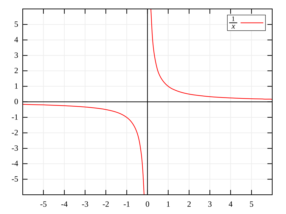
Graph of the function $y = 1/x$ showing a vertical asymptote at $x = 0$ . As $x$ approaches $0$ from the right, the curve rises toward $+\infty$ ; as $x$ approaches $0$ from the left, it falls toward $-\infty$ . The same graph also illustrates that the function values remain bounded away from zero as $|x|$ becomes large, a detail that goes slightly beyond the current syllabus focus on behavior near the asymptote. Source.

A well-scaled graph is essential because inappropriate scaling can hide steep growth or decay. If the graph appears flattened or compressed, true unbounded behavior may not be immediately obvious. Students must remain cautious and consider whether the displayed window accurately reflects the function’s behavior close to the point of interest.

Describing Unbounded Behavior Using Formulas

Algebraic expressions reveal unbounded behavior by showing how a function responds as the input nears values that make denominators zero or drive expressions to extreme magnitudes.

Analytical Signals of Unboundedness

A formula may indicate unbounded behavior when:

A denominator approaches zero while the numerator remains nonzero.
A function includes terms that grow extremely large for inputs near a specific value.
An expression produces values that oscillate widely while overall magnitude becomes unbounded.

These indicators must be connected to infinite limits, which formally describe unbounded function values.

Infinite Limit: A limit in which function values increase or decrease without bound as the input approaches a number.

Once a student identifies a structural cause of unbounded growth or decay in a formula, they can translate this observation into proper limit notation.

$\lim_{x \to a} f(x) = \infty$
$f(x)$ = Function whose values increase without bound
$a$ = Input value toward which $x$ approaches

Normal sentence: This notation captures the idea that although function values do not converge to a finite number, their behavior is still predictable and meaningful.

Relating Graphs and Formulas to Limits Involving Infinity

This syllabus requirement stresses the importance of synthesizing visual and algebraic information when interpreting unbounded behavior. Students must understand that infinite limits describe how a function behaves, not whether a function reaches infinity as a numerical value. Functions never “equal” infinity; rather, they exhibit outputs that grow beyond all finite bounds.

How Limits Formalize Graphical Behavior

When a graph rises sharply near a value of $x$ , we formalize that with limit notation indicating divergence to positive infinity. When the graph falls sharply, the corresponding limit involves negative infinity. Graphs that show different behaviors on opposite sides of a vertical asymptote require separate one-sided limits.

How Formulas Predict Graphical Behavior

Algebraic structures reveal the direction of divergence:

If a denominator approaches zero while remaining positive, the expression may diverge to $\infty$ .
If it approaches zero while remaining negative, the expression may diverge to $-\infty$ .
If numerator and denominator interact in complex ways, factoring or sign analysis clarifies the outcome.

Each of these analytic insights must connect to specific slope and curvature patterns visible on a graph.

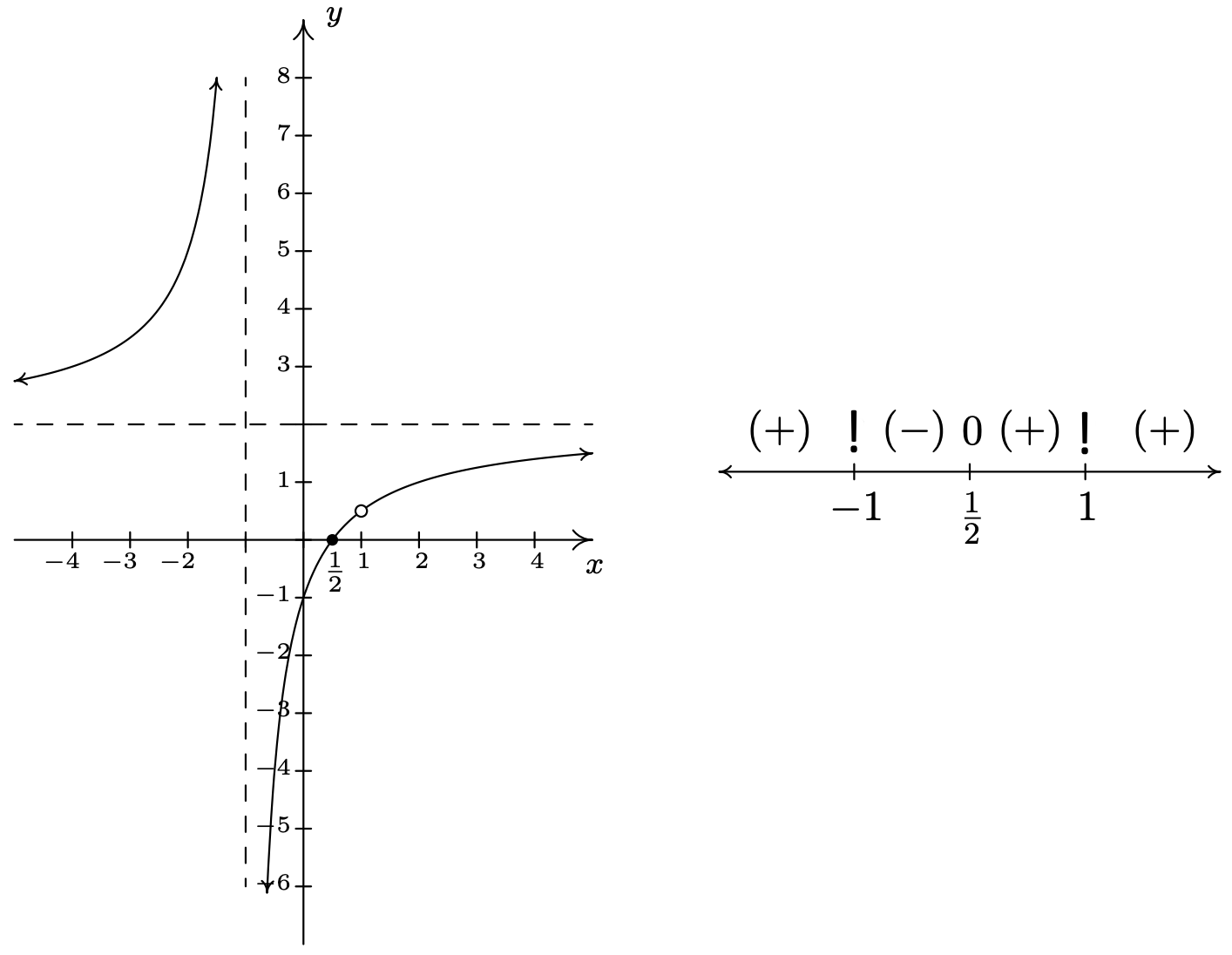
Graph of a rational function $y = h(x)$ with a vertical asymptote at $x = -1$ , a hole at $x = 1$ , and a zero at $x = \tfrac{1}{2}$ . The curve approaches the vertical asymptote with unbounded behavior on each side, illustrating how infinite limits arise at domain exclusions. The accompanying sign diagram provides additional information not required by the AP Calculus AB syllabus for this subsubtopic. Source.

Integrating Multiple Representations

Understanding unbounded behavior requires the ability to:

Interpret steep curves or sharp drops on a graph.
Detect algebraic structures that generate unbounded outputs.
Translate both observations into formal limit statements involving $\infty$ or $-\infty$ .

This integration aligns directly with the syllabus emphasis on describing unbounded and asymptotic behavior in both graphical and analytic contexts.

FAQ

Unbounded behaviour occurs when the function values show no sign of levelling off and continue increasing or decreasing as the graph approaches a specific x-value.

To check this:
• Look for vertical alignment with a particular x-value that the graph never crosses.
• Examine whether values appear to double, triple, or grow rapidly within small horizontal intervals.
• If zooming in reveals the graph still rising or falling without approaching a plateau, the behaviour is likely unbounded.

This often results from the algebraic structure of the function, especially the signs of numerator and denominator terms.

For example, if the denominator approaches zero with opposite signs depending on direction, the output may tend to positive infinity from one side and negative infinity from the other.

This directional dependence makes one-sided limits crucial for accurately describing the behaviour.

Yes. Vertical asymptotes are the most common cause, but other structures can create unboundedness.

Examples include:
• Highly oscillatory functions whose amplitude grows near a point.
• Functions defined piecewise where one branch grows without bound as it nears the boundary.

In such cases the behaviour still counts as unbounded, even if no simple line x = a formally acts as an asymptote.

Tables allow you to observe the numerical trend directly without relying on the graph’s scaling.

To use a table effectively:
• Check whether values grow extremely large in magnitude as x approaches a fixed point.
• Compare values from both sides; sudden sign changes or dramatic magnitude increases indicate unboundedness.

Tables are especially useful when the graph window hides steep vertical changes.

A frequent misconception is assuming that a graph going off-screen always means unbounded behaviour; sometimes it is merely poorly scaled.

Other pitfalls include:
• Thinking the function “reaches” infinity, rather than recognising infinity as a description of behaviour.
• Assuming both sides of a point must behave the same way. They may diverge differently.
• Confusing removable discontinuities with unbounded behaviour; removable discontinuities do not involve divergence.

Practice Questions

Question 1 (1–3 marks)
The graph of a function f shows that as x approaches 2 from both sides, the function values decrease without bound.
(a) State the type of behaviour the function exhibits near x = 2.
(b) Write a limit statement that describes this behaviour.

Question 1
(a) 1 mark
• Identifies unbounded behaviour or states that the function tends to negative infinity.
(b) 1–2 marks
• Writes an appropriate limit statement, for example:
lim f(x) = -∞ as x approaches 2. (1 mark)
• Statement must indicate the limit is the same from both sides. (1 mark)

Question 2 (4–6 marks)
A function g is defined for all x except x = 3. The table below shows selected values of g(x):

x: 2.8, 2.9, 2.95, 3.05, 3.1, 3.2
g(x): 12, 25, 60, -55, -28, -15

(a) Describe the unbounded behaviour of g as x approaches 3 from the left.
(b) Describe the unbounded behaviour of g as x approaches 3 from the right.
(c) Explain what the behaviour in parts (a) and (b) suggests about the presence of an asymptote.

Question 2
(a) 1–2 marks
• States that as x approaches 3 from the left, g(x) increases without bound or becomes very large and positive. (1 mark)
• Uses correct terminology such as unbounded behaviour or divergence. (1 mark)

(b) 1–2 marks
• States that as x approaches 3 from the right, g(x) decreases without bound or becomes very large in the negative direction. (1 mark)
• Uses correct terminology such as unbounded behaviour or divergence. (1 mark)

(c) 1–2 marks
• States that the behaviour suggests a vertical asymptote at x = 3. (1 mark)
• Provides justification referencing opposite unbounded behaviour on each side of x = 3. (1 mark)

Try All Topic Practice Questions

Written by:

Dr Rahil Sachak-Patwa

Oxford University - PhD Mathematics

Rahil spent ten years working as private tutor, teaching students for GCSEs, A-Levels, and university admissions. During his PhD he published papers on modelling infectious disease epidemics and was a tutor to undergraduate and masters students for mathematics courses.