Understanding how to interpret analytic limit notation helps reveal a function’s nearby behavior, allowing students to connect symbolic expressions to graphical trends and numerical patterns.

Interpreting Analytic Limit Notation

Analytic limit notation communicates how a function behaves near a point rather than what the function equals at that point. When students see an expression such as $\lim_{x\to c} f(x) = L$, the notation is describing an approach, not a substitution. This perspective is central to early calculus and underpins later ideas about continuity and derivatives, making careful interpretation essential.

What Limit Notation Communicates

A written limit gives a verbal description of behavior, specifying what $f(x)$ is getting close to as $x$ gets arbitrarily near a specific number $c$. It does not claim that $f(c)$ exists or that $f(c)=L$. Instead, the notation highlights the trend of nearby values, which is often clearer when linked to graphs or tables of values.

Interpreting analytic limit statements requires distinguishing between function value and approaching value, as these may differ significantly in piecewise or discontinuous contexts.

Connecting Notation to Verbal Descriptions

Analytic notation should always be translatable into meaningful language. A limit statement like $\lim_{x\to 3} f(x)=5$ means: “As $x$ gets arbitrarily close to 3, the values of $f(x)$ get arbitrarily close to 5.” When students convert notation to words, they reinforce the idea of approach without necessarily reaching, which avoids the common misconception that limits require substitution.

Bullet points can help capture the layered interpretation of a limit statement:

• The input value approaches a number $c$.

• The output values move toward a single number $L$.

• The function’s value at $c$ may be equal to $L$, not equal to $L$, or even undefined.

• The notation describes nearby behavior, not behavior at the point itself.

These verbal interpretations prepare students to connect notation to multiple representations and to reason about limits without relying exclusively on algebraic expressions.

Linking Notation to Graphical Behavior

Graphs visually demonstrate the meaning of analytic limit notation by showing how $f(x)$ behaves around $x=c$. To interpret analytic notation graphically, students should focus on the y-values approached rather than the plotted point at $x=c$. This supports the understanding that the limit depends on what the function is doing close to that point, even if the graph has a hole or jump.

When interpreting $\lim_{x\to c} f(x)=L$ from a graph:

• Look at the left-hand behavior, observing the outputs for x<c approaching $c$.

• Examine the right-hand behavior, observing the outputs for x>c approaching $c$.

• Confirm both sides approach the same y-value $L$.

• Ignore the actual plotted value at $x=c$, since the limit concerns surrounding behavior.

Understanding these graphical cues helps students validate analytic limit statements and recognize when a limit does not match the function's value.

Graphs visually demonstrate the meaning of this notation: as you move along the curve closer to x=cx = cx=c from either side, the yyy-values should settle near LLL.

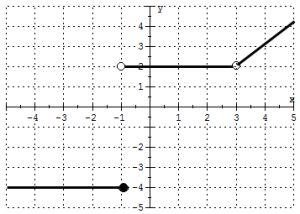
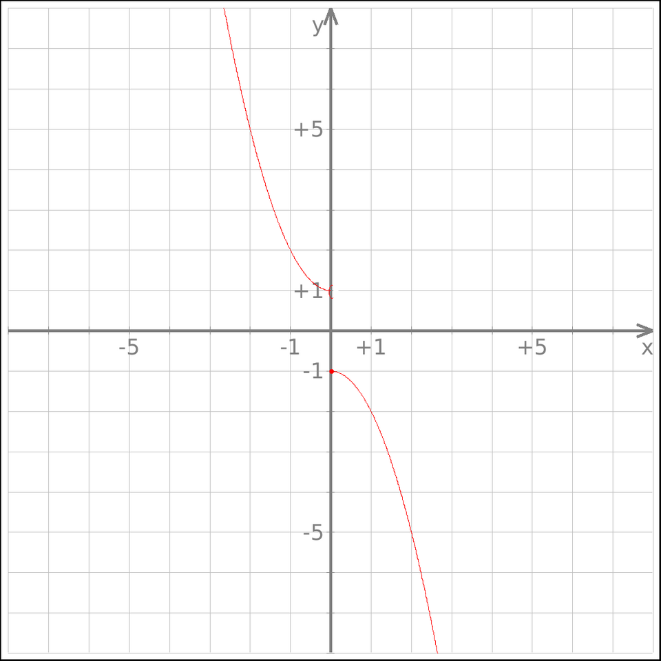
Graph of a piecewise function with an open circle where the function is not defined and a filled point at a different height. The graph illustrates that the limit as xxx approaches a point is determined by the values approached from each side, even when f(c)f(c)f(c) is missing or different. Parts of the graph away from the highlighted open and closed circles include extra detail not required by the syllabus and can be de-emphasized when teaching. Source.

Linking Notation to Numerical Patterns

Tables of values also provide a complementary perspective on analytic limit notation. When interpreting notation numerically, students analyze patterns in function values as $x$ approaches $c$ from both sides. Numerical interpretation is especially useful when formulas are difficult to manipulate or when graphs are not provided.

To translate analytic notation into numerical reasoning:

• Identify $x$-values close to but not equal to $c$.

• Observe how the corresponding $f(x)$ values behave as $x$ moves closer to $c$.

• Determine whether values appear to settle near a single number that matches the analytic limit statement.

• Recognize inconsistencies—such as divergence or differing left-hand and right-hand trends—as indicators that the limit notation may not describe the function accurately.

These numerical patterns reinforce the interpretation of limit notation as a statement about approach, not exactness.

Integrating Multiple Representations Through Analytic Notation

A powerful interpretation of analytic limit notation comes from synthesizing symbolic, graphical, and numerical viewpoints. This synthesis allows students to confirm whether the analytic statement accurately reflects the function's true behavior. It also encourages flexible thinking, a crucial skill in calculus.

Students should be able to:

• Translate $\lim_{x\to c} f(x)=L$ into precise verbal explanations.

• Use a graph to justify that the behavior near $x=c$ aligns with the analytic claim.

• Reference numerical evidence as further support when needed.

• Identify when an analytic statement contradicts graphical or numerical patterns.

Through this integrated approach, analytic limit notation becomes more than a symbolic expression; it becomes a concise summary of how a function behaves near a specific point, supported by multiple forms of evidence.

If the left-hand and right-hand limits are not equal, we write that the limit lim⁡x→cf(x)\lim_{x\to c} f(x)limx→c​f(x) does not exist (DNE), even if each one-sided limit individually exists.

Graph of a function with a jump discontinuity: as xxx approaches a point from the left, the graph approaches one yyy-value, while from the right it approaches a different value. This visually encodes the notation lim⁡x→c−f(x)\lim_{x\to c^-} f(x)limx→c−​f(x) and lim⁡x→c+f(x)\lim_{x\to c^+} f(x)limx→c+​f(x) and shows why the combined limit lim⁡x→c\lim_{x\to c}limx→c​ does not exist. Additional portions of the curve beyond the jump appear in the diagram but are not required by the syllabus. Source.