
AP Syllabus focus:
‘Translate information about limits among graphs, tables, and analytic expressions, ensuring the same limit behavior is accurately represented in different forms.’
Understanding how limit behavior appears in graphs, tables, and formulas builds essential flexibility in analyzing functions. This subsubtopic emphasizes translating limit information accurately across representations.
Understanding Limit Behavior Across Representations
Limit problems often present information in different forms, yet they describe the same underlying behavior: how a function behaves near a point, not necessarily at the point. Being able to move among these forms strengthens conceptual understanding and prevents overreliance on a single representation.
When discussing such behavior, the limit of a function refers to the value the function’s outputs approach as the input gets arbitrarily close to a chosen number.
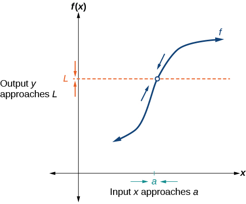
A graph illustrating a function approaching a limit L as x approaches a, with a hole at (a, L) to emphasize that the limit depends on nearby behavior rather than the function’s value at that point. Source.
Limit of a function: The value a function’s outputs approach as the input gets arbitrarily close to a chosen number.
This concept is central when translating information from one form to another because each representation illustrates the function’s approach in its own way.
Reading Limit Behavior from Graphs
Graphs offer a visual perspective on limit behavior. Students must examine the function’s y-values as the graph approaches an x-value from both the left and right.
Key Observations from Graphs
Identify the approach behavior, not just the point’s plotted value.
Look for agreement between the left-hand behavior and right-hand behavior.
Note whether holes, jumps, or asymptotes affect the function’s local behavior.
These observations guide the translation of graphical information into formal limit notation or into a numerical table that reflects the same behavior.
Translating Graphs into Tables
A numerical table mirrors what the graph shows by listing x-values approaching a target from both sides.
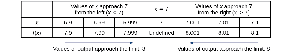
A table showing x-values approaching 7 from both sides and corresponding f(x) values approaching 8, illustrating how numerical data can reveal a limit even when the function is undefined at the target point. Source.
When converting graphical information to tabular form, focus on selecting x-values that capture the trend shown visually.
Building a Consistent Table
Choose x-values that get progressively closer to the target point from the left.
Choose a symmetric or similarly close set of values from the right.
Record the corresponding y-values suggested by the graph’s trend.
Even though exact values may not be given visually, the behavior implied by the graph determines what should appear numerically in the table.
Translating Tables into Formulas or Limit Statements
Tables provide approximate values that suggest a limiting value. Converting this to analytic notation requires interpreting what the table implies about the function.
Indicators from Tables
Values that stabilize suggest a finite limit.
Values trending upward or downward may indicate an infinite limit.
Disagreement between left and right approaches suggests the limit does not exist.
These interpretations then translate into a symbolic statement about function behavior.
Limit notation: A formal symbolic expression describing the value a function approaches as the input approaches a specified point.
Writing a limit statement after examining a table ensures the symbolic form accurately reflects numerical behavior.
Expressing Graphical or Tabular Behavior with Formulas
Sometimes the underlying functional rule is known, but the graphical or numerical behavior must still match the limiting behavior implied by the rule. A formula can be examined directly using substitution or algebraic reasoning, but the limit behavior it predicts must also be representable in graphical and tabular forms.
Ensuring Alignment Across Representations
A hole in the graph corresponds to an undefined value in the formula but does not affect the limit if the nearby values approach a single number.
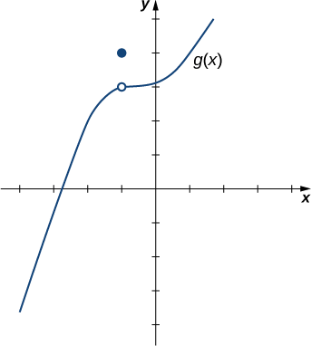
A graph showing a function with a hole at one y-value and a different defined point at the same x-value, illustrating how the limit is determined by the curve’s approach rather than the function’s actual value at that point. Source.
A jump in the graph signals a mismatch in left- and right-hand behavior and should appear in tables as differing approach values.
A vertical asymptote corresponds to values in tables growing without bound and to unbounded behavior in the graph.
Ensuring alignment means all three representations must tell the same story about how the function behaves near the point of interest.
Using Analytic Expressions to Infer Graphs and Tables
Formulas can often be analyzed to predict the type of behavior expected in other representations. When performing such translations, pay attention to the structural features of the expression.
Structural Clues from Formulas
Factorable expressions may show removable features, leading to smooth graphical approaches.
Expressions with denominators approaching zero may indicate unbounded behavior.
Piecewise-defined expressions may reveal differing local behaviors depending on direction.
These structural patterns should then be expressed visually in a graph or numerically in a table.
= Input approaching the value (no units)
= Limit value approached by near (depends on context)
A sentence must follow here to ensure proper spacing between equation blocks and the rest of the text, reinforcing clarity and readability for students.
Strategies for Accurate Conversion Among Representations
When moving between graphs, tables, and formulas, consistency is key. Students should ensure that all representations communicate the same limiting behavior.
Effective Strategies
Compare left-hand and right-hand behaviors carefully in each representation.
Maintain focus on approach behavior rather than the function’s value at the point.
Ensure numerical tables become tighter around the point when refining the limit estimate.
Check that symbolic expressions support the trends observed graphically and numerically.
These strategies help guarantee accurate translation and deepen understanding of limit behavior across mathematical representations.
Practice Questions
Question 1 (1–3 marks)
A function f is represented by the graph of a curve. As x approaches 2 from both sides, the y-values of the curve appear to approach 5, even though the point (2, 3) is filled in on the graph.
(a) State the value of lim f(x) as x approaches 2.
(b) Explain briefly why the value of f(2) does not affect the limit.
Question 1 (1–3 marks)
(a) 1 mark
• Correct answer: 5.
(b) Up to 2 marks
• 1 mark for stating that the limit depends on values close to x = 2, not the function’s value at x = 2.
• 1 mark for noting that the filled point (2, 3) does not change the approach of the graph towards 5.
Question 2 (4–6 marks)
A function g is defined for all x ≠ 1. The table below gives values of g(x) for x near 1.
x: 0.8 0.9 0.99 1.01 1.1 1.2
g(x): 3.4 3.7 3.9 4.1 4.3 4.6
(a) Use the table to estimate lim g(x) as x approaches 1.
(b) Describe how the table indicates whether the left-hand and right-hand behaviours agree.
(c) Suggest one graphical feature that a corresponding graph of g might display at x = 1, based on the information provided.
(d) Explain how the limit value, rather than g(1), determines the behaviour illustrated in the table.
Question 2 (4–6 marks)
(a) 1 mark
• Correct estimate: approximately 4 (accept any value between 3.9 and 4.1).
(b) Up to 2 marks
• 1 mark for noting that values from the left (0.8, 0.9, 0.99) approach about 4.
• 1 mark for noting that values from the right (1.01, 1.1, 1.2) also approach about 4.
(c) Up to 2 marks
• 1 mark for identifying a hole or removable discontinuity.
• 1 mark for explaining that this is suggested because the limit exists but g(1) is not defined.
(d) 1 mark
• Correct explanation that the table reflects the behaviour of g near x = 1, and therefore the limit captures the overall trend regardless of the value (or absence of a value) at x = 1.
FAQ
A graph is reliable for estimating a limit only if it shows clear behaviour extremely close to the target x-value. If the scale is coarse or the resolution low, apparent trends may be misleading.
Check whether:
• The axes include sufficiently fine increments.
• The plotted curve has no missing sections near the point.
• Left-hand and right-hand traces visibly approach the same height.
If uncertainty remains, support the graph with a table or analytic reasoning.
Numerical tables may give inconsistent values if the chosen x-values are too far from the target or if rounding errors distort the outputs.
To improve reliability:
• Use x-values substantially closer to the target point.
• Reduce step size between successive entries.
• Compare left-hand and right-hand lists for symmetry.
Well-constructed tables should show convergence towards a single value.
Cross-verification is key. Each representation should indicate the same limiting behaviour independently.
A strong confirmation occurs when:
• The graph shows both sides approaching the same height.
• The table gives values stabilising near that height.
• The formula, when simplified, predicts a consistent limit.
If any representation conflicts, re-examine scaling, computation, or algebraic manipulation.
Ambiguity arises when the graph lacks clarity around the point of interest.
Warning signs include:
• Overlapping curves or cluttered plotting.
• Sudden changes in steepness close to the target x-value.
• Missing open or closed markers that would clarify function values.
In such cases, rely on numerical tables or algebraic analysis rather than the graph alone.
Certain algebraic forms naturally create misleading visuals or numerical instability.
Examples include:
• Expressions with factors that cancel, producing a hole not obvious from the unsimplified formula.
• Very steep slopes near the target point, causing tables to fluctuate unless x-values are extremely close.
• Complex rational forms where tiny denominator values exaggerate small numerical errors.
Identifying these features helps interpret graphs and tables more accurately.
