
AP Syllabus focus:
‘Represent derivatives using tables and graphs, including matching a function with the graph of its derivative and estimating derivative values from these representations.’
Understanding how to represent derivatives numerically and graphically helps connect the algebraic definition of the derivative to observable patterns in tables and visual features in graphs.
Representing Derivatives Numerically
Numeric representations rely on data organized in a table to approximate how a function changes. These approximations help students identify where a function is increasing, decreasing, or changing rapidly.
Using Tables of Function Values
A table of inputs and outputs reveals how the function behaves locally. When values are close together, the table becomes a powerful tool for estimating the instantaneous rate of change, which is the derivative at a point.
Instantaneous Rate of Change: The rate at which a function changes at a single input value, found as the limit of average rates of change over shrinking intervals.
Because tables present discrete information, students focus on average rates of change over small intervals to approximate derivative values. Smaller intervals generally lead to better approximations, provided the function behaves smoothly near the point of interest.
Estimating Derivatives with Difference Quotients
A difference quotient uses nearby function values to estimate the slope. When symmetric intervals are available, students obtain a more balanced approximation that reduces directional bias.
Symmetric Difference Quotient(a) = ( f(a + h) – f(a – h) ) / (2h)
a = Input at which the derivative is approximated
h = Small step size from the input
Because numerical approximations depend on the quality and density of available data, students must evaluate whether the table offers sufficiently close points to model local behavior.
Representing Derivatives Graphically
Graphs provide a visual illustration of how a derivative behaves by connecting the geometry of the curve to the slope of a tangent line at each point.
Tangent Line Interpretation
The derivative represents the slope of the tangent line, a geometric feature indicating the function’s instantaneous direction and steepness.
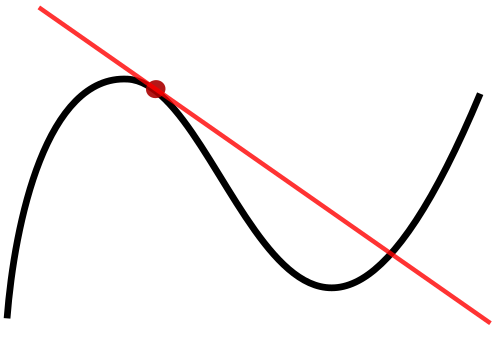
A differentiable curve (black) with its tangent line (red) illustrates how the slope of the tangent represents the derivative at that point, emphasizing local linear approximation. Source.
Tangent Line: A line that touches a curve at exactly one point and has the same instantaneous direction as the curve at that point.
When viewing a graph, steep upward segments correspond to positive derivative values, whereas steep downward segments correspond to negative values. Flat points on the graph indicate a derivative of zero.
Matching a Function to its Derivative Graph
Students must identify patterns that connect the shape of the original function to features of the derivative graph. Key relationships include:
Where the function is increasing, the derivative graph lies above the x-axis.
Where the function is decreasing, the derivative graph lies below the x-axis.
Where the function has a local maximum or minimum, the derivative crosses the x-axis.
Sharp changes in steepness appear as sudden height changes in the derivative graph.
These connections help students reason backward or forward between representations without relying on algebraic differentiation.
Using Slopes of Secant Lines on Graphs
Graphical representations often allow students to estimate slopes visually by drawing secant lines, which approximate the slope near a point using two close points on the curve. As the points move closer, the secant line slope approaches the tangent slope, reinforcing the conceptual link between average and instantaneous rates.
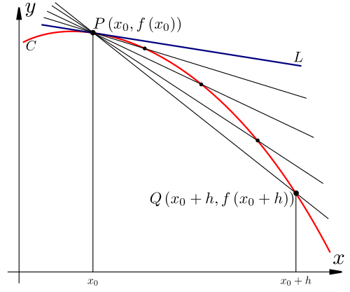
A curve with its tangent and a family of secant lines shows how secant slopes converge to the derivative as h approaches zero, visually illustrating the limiting process. Source.
Secant Slope = ( f(b) – f(a) ) / (b – a)
a, b = Inputs used to approximate local behavior
Because graphs may not provide perfectly precise information, these slope estimates are approximate, yet they reveal trends consistent with the function’s overall behavior.
Interpreting Derivative Values from Representations
Interpreting derivative values numerically or graphically strengthens students’ conceptual understanding of how functions change. Each representation highlights different features:
Tables emphasize localized numeric changes in outputs.
Graphs reveal broad structural patterns such as critical points and intervals of monotonicity.
Slope analysis connects numeric patterns to geometric interpretations.
Recognizing the Derivative as Its Own Function
When derivative values are collected—either from tables or from tangent line slopes on graphs—they form a new function, f′(x), whose behavior describes how the original function changes. Students should view this derivative graph as a standalone representation governed by the same principles of continuity and slope interpretation that apply to the original function.
Combining Numerical and Graphical Reasoning
Effective analysis involves synthesizing information across representations. Students deepen understanding when they:
Examine how steepness in the graph corresponds to the size of numeric slopes.
Predict derivative graph behavior before viewing it.
Compare numeric estimates to features such as increasing/decreasing intervals.
These strategies foster a stronger conceptual grasp of derivatives beyond procedural calculations, aligning with the goal of representing derivatives using tables and graphs.
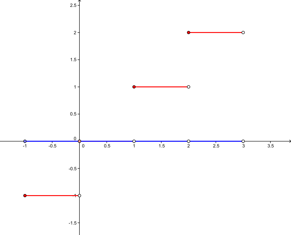
A step function and its derivative display how constant intervals correspond to derivative values of zero, while jump discontinuities create points where the derivative does not exist, reinforcing graphical interpretation principles. Source.
Practice Questions
Question 1 (1–3 marks)
A function f is shown in a table of values for x near 2.
x: 1.8, 1.9, 2.1, 2.2
f(x): 3.2, 3.5, 4.1, 4.6
(a) Use an appropriate difference quotient to estimate f ’(2).
(b) State whether your estimate suggests the graph of f is increasing or decreasing at x = 2.
Question 1
(a) 2 marks
• 1 mark for choosing a valid symmetric or one-sided difference quotient using values near x = 2.
• 1 mark for a correct numerical estimate.
(b) 1 mark
• 1 mark for stating that the function is increasing if the estimate is positive, or decreasing if it is negative, with a brief justification.
Total: 3 marks
Question 2 (4–6 marks)
The graph of a differentiable function g is shown. At x = 1, the graph appears to have a tangent line with a positive, gradually increasing slope. Between x = 2 and x = 4, the graph flattens before decreasing sharply after x = 4.
(a) Sketch a possible graph of g ’(x) over the interval 0 ≤ x ≤ 5, labelling key features.
(b) Identify one interval where g ’(x) is positive and one interval where g ’(x) is negative, explaining how you know.
(c) Estimate the value of g ’(1) based on the behaviour of the tangent line described.
Question 2
(a) 2 marks
• 1 mark for sketching g ’(x) above the x-axis where g is increasing and below the x-axis where g is decreasing.
• 1 mark for indicating g ’(x) close to zero where the graph of g flattens.
(b) 2 marks
• 1 mark for identifying an interval where g ’(x) is positive with correct reasoning.
• 1 mark for identifying an interval where g ’(x) is negative with correct reasoning.
(c) 1–2 marks
• 1 mark for a reasonable positive estimate of the slope at x = 1.
• 1 mark for a clear explanation referring to the tangent line’s increasing slope.
Total: 5–6 marks
FAQ
Uneven spacing does not prevent derivative estimation, but it affects which difference quotient is most reliable. Symmetric differences are only valid when points are equally spaced around the target value.
When spacing is uneven, use the closest forward or backward difference instead. The accuracy depends on:
• How close the points are to the target
• How smoothly the function behaves in that region
Smaller intervals usually give better estimates regardless of spacing.
Students often confuse the height of the graph with its slope. A function can be high above the axis yet still be decreasing.
Misidentifications typically arise from:
• Curves that level off subtly, causing slope changes to be overlooked
• Steep curves where visual estimation exaggerates the slope
• Points near turning points, where the slope changes sign rapidly
A reliable strategy is to imagine the tangent line rather than focusing on the curve’s vertical position.
Yes. A derivative graph indicates how quickly the slope of the function is changing. If the derivative varies sharply near the value you are estimating, small changes in x can lead to large differences in derivative estimates.
Tables are least reliable when:
• The derivative graph shows high curvature or rapid oscillation
• The function has near-cusp behaviour, even if not a true cusp
• The table provides points too widely spaced to reflect rapid changes
In such cases, more data or graphical verification is needed.
A nearly horizontal graph segment may mislead students into assuming the derivative is zero. To confirm:
• Check whether the graph is exactly flat or only gently sloping
• Look for subtle changes in height over equal horizontal intervals
• Use estimated secant slopes between nearby points
A true zero derivative occurs only when the tangent line is perfectly horizontal. Gentle curvature still indicates a non-zero slope.
The derivative graph reflects rates of change rather than absolute values, so variations in the original graph can appear less pronounced.
This happens because:
• Derivatives reduce large-scale vertical shifts to changes in slope
• Local bumps in the graph may translate into minor variations in the derivative
• Visual noise or small irregularities in a drawn curve often diminish when expressed as slope
A smoother derivative graph implies that the function’s changes occur gradually, even if its values fluctuate more dramatically.
