The tangent line captures how a function behaves locally, offering a linear approximation that reflects the function’s immediate rate of change at a specific point.

Tangent Lines and Derivatives at a Point

Understanding the Tangent Line Concept

A tangent line is a line that touches the graph of a function at exactly one point near which it reflects the graph’s local direction. The slope of this line represents how the function is changing at that instant. Because of this, the tangent line is deeply connected to the derivative, which quantifies instantaneous change.

In calculus, the tangent line provides a powerful tool for local linear modeling, helping describe behavior that may otherwise be complicated to compute directly.

The Derivative as the Slope of the Tangent Line

The derivative at a point measures the instantaneous rate of change of a function. At $x=a$, this derivative value, $f'(a)$, becomes the slope of the tangent line to the graph of $f$.

Since slope represents rise over run, the derivative expresses how rapidly the output changes relative to a small change in the input. This relationship is fundamental when connecting graphical behavior with symbolic computations.

“The derivative at $x = a$, written $f'(a)$, is the slope of the tangent line to the graph of $y = f(x)$ at the point $(a, f(a))$.”

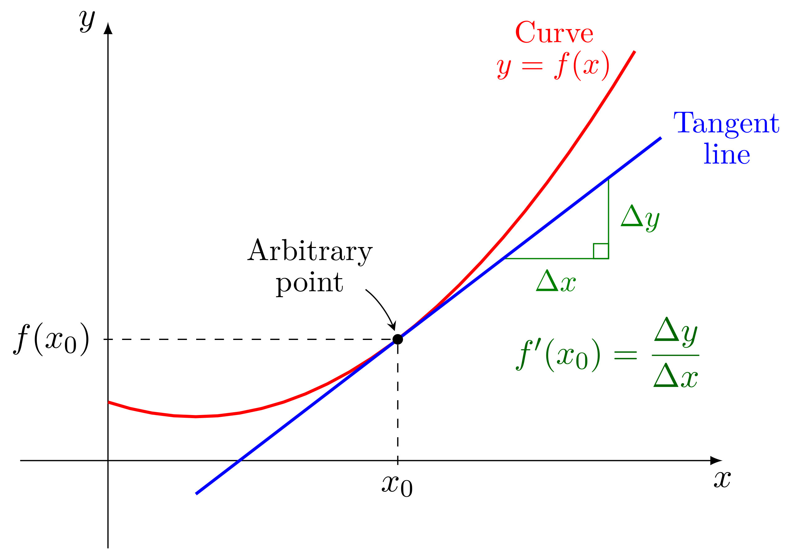
The curve $y=f(x)$ is shown with its tangent line at $x_0$, where the slope is illustrated using $\Delta x$ and $\Delta y$. The geometric relationship $f'(x_0)=\frac{\Delta y}{\Delta x}$ reinforces that the derivative represents the slope of the tangent line. This image visually supports the idea that instantaneous rate of change corresponds to the tangent line’s slope. Source.

Writing the Equation of a Tangent Line

When constructing the tangent line, we use point-slope form, which relies on knowing one point on the line and its slope. For a differentiable function $f$ at $x=a$, the point on the curve is $(a, f(a))$ and the slope is $f'(a)$.

Because point-slope form centers the equation around the specific point of tangency, it provides a precise representation of local linear behavior.

A tangent line equation is considered complete when all quantities are substituted, but for conceptual understanding, recognizing the structure is most important at this stage.

Why the Tangent Line Matters

The tangent line is not only a helpful geometric object but also a key analytical tool. Its importance stems from several features:

• It approximates the function near the point of tangency, aiding in interpretation and prediction.

• It encodes instantaneous change, which is essential in modeling motion, growth, and optimization.

• It bridges graphical understanding with algebraic structure, reinforcing the connection between shape and rate.

By examining how the tangent line sits relative to the graph, students can infer whether the function is increasing or decreasing and how rapidly these changes occur.

Visual and Analytical Characteristics of Tangent Lines

To fully understand tangent lines, it is useful to connect their analytic form to their geometric appearance.

Key ideas include:

• A positive derivative corresponds to an upward-sloping tangent line.

• A negative derivative corresponds to a downward-sloping tangent line.

• A zero derivative indicates a horizontal tangent, often found at local maxima or minima.

• The steepness of the line reflects the magnitude of the derivative; the larger the absolute value of $f'(a)$, the steeper the tangent.

These characteristics allow students to move fluidly between the algebraic computation of derivatives and visual interpretations on graphs.

Steps for Constructing and Interpreting Tangent Lines

To ensure clarity when working with tangent lines, students should follow a structured approach:

• Identify the point of tangency $x=a$ and compute $f(a)$.

• Determine the derivative $f'(a)$ to obtain the slope.

• Substitute values into the point-slope form.

• Interpret how the tangent line reflects local behavior of the original function.

This layered process keeps the emphasis on the connection between derivative values and geometric meaning.

Relationship Between Local Linearization and Tangent Lines

Because the tangent line models a function near a single point, it plays a central role in local linearization, a technique used to approximate function values close to $x=a$. Even though full applications extend beyond this subsubtopic, recognizing that the tangent line acts as the function’s best linear approximation underscores its conceptual value.

“Near $x = a$, the tangent line provides a local linear approximation to $f$, so its values stay close to the actual function values for inputs near $a$.”

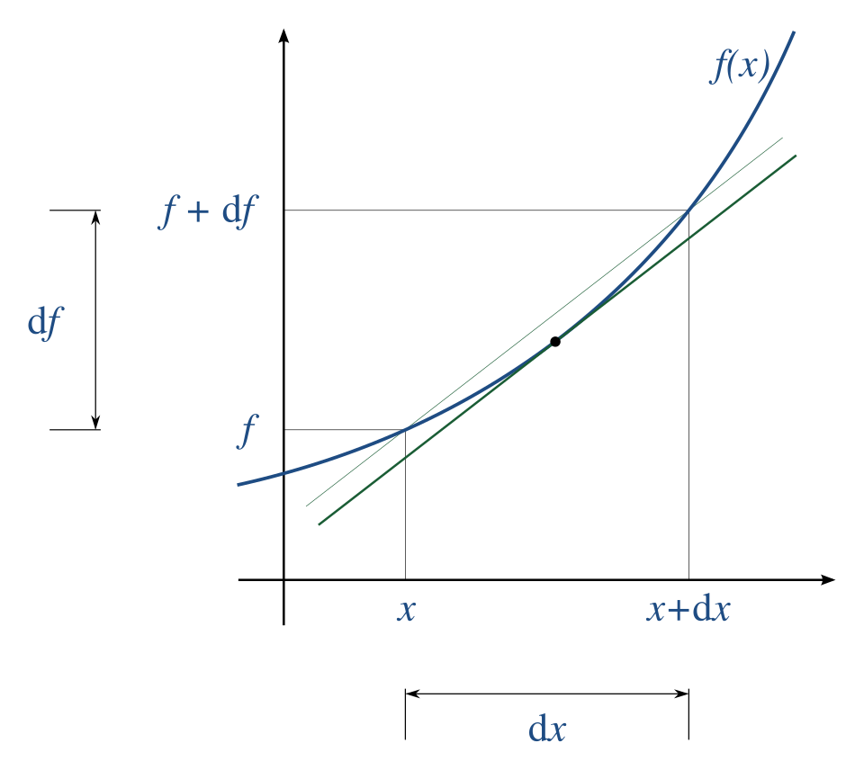
The curve $f(x)$ is shown with its tangent line and nearby points at $x$ and $x+dx$, illustrating changes $dx$ and $df$. The slope $\frac{df}{dx}$ matches the tangent line’s slope, emphasizing the derivative as a measure of instantaneous change. Labels such as $df$ and $dx$ exceed AP requirements but visually reinforce the idea of local linear approximation. Source.

Situations Where Tangent Lines Provide Insight

Students encounter tangent lines in several contexts within calculus:

• Interpreting instantaneous velocity in motion problems.

• Assessing sensitivity or marginal change in economic models.

• Understanding the shape of a graph in relation to its increasing or decreasing behavior.

• Predicting the direction of a function’s change at specific input values.

By tying together these ideas, tangent lines become one of the most versatile and foundational tools in the study of differentiation.