
AP Syllabus focus:
‘Combine the power rule with constant multiple, sum, and difference rules to find derivatives of polynomial functions efficiently without returning to the limit definition.’
Polynomial differentiation builds on earlier derivative rules to create a highly efficient process. By combining structured rules, students compute derivatives rapidly while maintaining conceptual clarity.
Understanding Polynomial Structure
Polynomial expressions are built from terms, each consisting of a constant coefficient multiplied by a variable raised to a real exponent. Because polynomials combine multiple terms through addition or subtraction, differentiation requires a rule-based, term-by-term approach that avoids the limit definition.
The Role of the Power Rule
The power rule serves as the foundation for differentiating each term Individually within a polynomial. Applied consistently, it transforms expressions involving powers of into simpler forms that capture instantaneous rates of change within algebraic models.
Power Rule: For any differentiable function of the form , its derivative is obtained by multiplying by the exponent and reducing the exponent by one.
Before applying this rule, it is essential to recognize that polynomial terms may possess positive, negative, or zero exponents and may include scalar coefficients.
Essential Derivative Rules Used with Polynomials
Polynomial differentiation relies on a structured combination of rules that operate seamlessly together.
Constant Multiple Rule
This rule allows a constant factor to remain unchanged during differentiation while the derivative applies only to the variable expression.
Constant Multiple Rule: If is constant and is differentiable, then the derivative of equals times the derivative of .
These rules function intuitively: constants scale the slope of the function but do not alter how the variable term behaves.
Sum and Difference Rules
Because polynomials combine several terms, these rules enable differentiation of each term independently.
Sum and Difference Rules: The derivative of equals the derivative of plus or minus the derivative of .
This structure ensures that differentiation distributes across the polynomial, supporting efficiency and accuracy.
Applying Rules Systematically to Polynomial Expressions
Differentiation of polynomials is inherently procedural. Each term is processed independently, producing a new polynomial that represents the instantaneous rate of change of the original function.
Steps for Differentiating Polynomial Functions
Students should apply the following logical sequence:
Identify each term in the polynomial and determine its exponent and coefficient.
Apply the power rule to variable expressions.
Use the constant multiple rule to keep coefficients attached during differentiation.
Use sum and difference rules to combine differentiated terms.
Ensure the final expression is simplified into standard polynomial form.
Because polynomials are differentiable across all real numbers, their derivatives also remain well-defined polynomials, simplifying subsequent analysis.
A short equation representation helps highlight how these rules collectively shape the derivative of a polynomial.
= polynomial function of degree
= constant coefficients
This general form illustrates how each term is prepared for differentiation using the same systematic principles.
Written in standard form, a polynomial function in one variable is a sum of constant multiples of powers of with nonnegative integer exponents.

General form of a polynomial function written as a sum of terms akxka_k x^kakxk with coefficients aka_kak and nonnegative integer exponents. This representation highlights the structure that allows each term to be differentiated using the power rule and the constant multiple rule. The image includes extra notation indicating the leading coefficient and degree, reinforcing terminology used when differentiating polynomial functions. Source.
Efficiency and Avoidance of the Limit Definition
One purpose of this subsubtopic is to highlight that polynomial differentiation does not require revisiting the limit definition of the derivative. Instead, previously established rules streamline the process without sacrificing rigor.
Why the Limit Definition Is No Longer Needed
Once the power rule and linearity properties (sum, difference, constant multiple) are established, they serve as complete tools for differentiating any polynomial. The limit definition remains conceptually important, but its repeated application becomes unnecessary for computational purposes. Students build fluency by applying rule-based shortcuts that preserve the meaning of the derivative while improving speed and accuracy.
Interpreting the Structure of Derivatives of Polynomial Functions
Once a polynomial is differentiated, the resulting expression provides insight into how rates of change behave across the function’s domain. Because derivatives of polynomials reduce their degree by one, the new function often displays simpler behavior while still capturing essential features.
Key Observations
The derivative of a polynomial is always another polynomial.
The degree decreases by one unless the original polynomial is constant.
Coefficients and exponents adjust predictably according to the rules.
Term-by-term differentiation reinforces algebraic comprehension and supports later applications such as optimization and motion modeling.
Consequently, the derivative of a polynomial is itself a polynomial whose degree is usually one less than the degree of the original function.
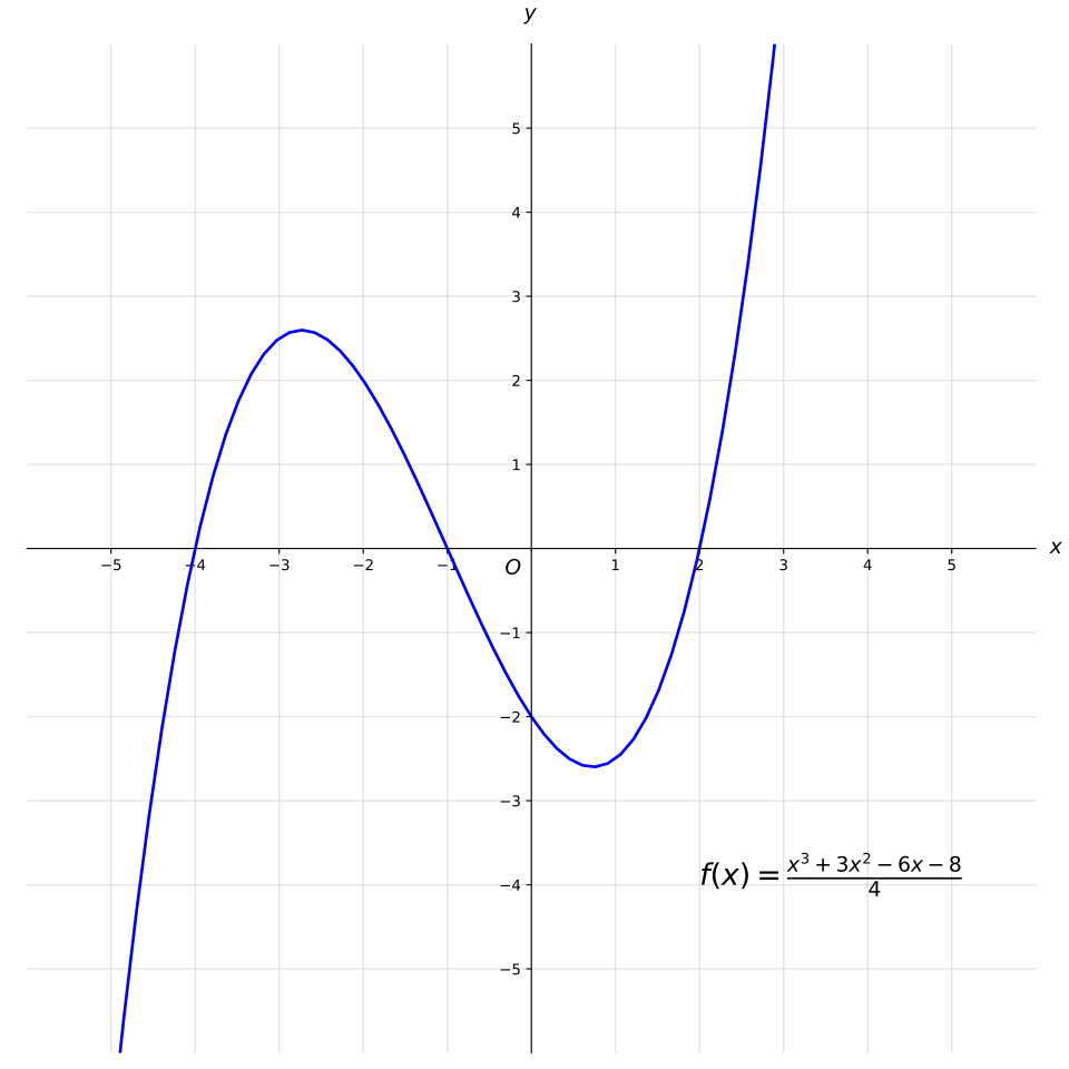
Graph of a degree-three polynomial illustrating smooth curvature and turning points. Differentiating this function yields a quadratic polynomial whose graph describes the slope of the cubic at each xxx-value. The image displays only the curve and axes, without extra details beyond what is required for this topic. Source.
This derivative polynomial gives the slope of the original graph at each -value and controls where the function is increasing, decreasing, or has horizontal tangents.
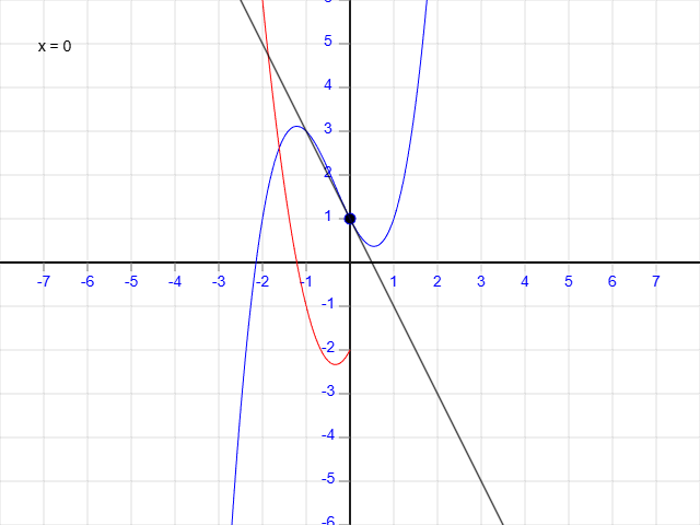
Graph showing a cubic polynomial f(x)=x3+ax2+bx+cf(x) = x^{3} + ax^{2} + bx + cf(x)=x3+ax2+bx+c in blue, its derivative f′(x)f'(x)f′(x) in red, and a tangent line in black at a movable point. As the point moves, the slope of the tangent and corresponding value on the derivative graph change simultaneously. The image contains additional parameter controls beyond the syllabus, included only because no simpler version of this paired polynomial–derivative graph was available. Source.
Practice Questions
Question 1 (1–3 marks)
A polynomial is defined by f(x) = 7x^4 − 3x^2 + 5x − 12.
(a) Differentiate f(x).
(b) State the degree of f ’(x).
Question 1
(a) f ’(x) = 28x^3 − 6x + 5
• 1 mark for correctly applying the power rule to 7x^4
• 1 mark for correctly differentiating the remaining terms
(b) Degree of f ’(x) is 3
• 1 mark for correct degree
Question 2 (4–6 marks)
A function is defined by g(x) = 4x^5 − 6x^3 + x.
(a) Find g ’(x).
(b) For what value(s) of x is the gradient of g(x) equal to 0?
(c) Explain what the result in part (b) indicates about the behaviour of g(x), giving a brief interpretation in terms of polynomial derivatives.
Question 2
(a) g ’(x) = 20x^4 − 18x^2 + 1
• 1 mark for differentiating 4x^5
• 1 mark for differentiating −6x^3
• 1 mark for differentiating x and assembling the full derivative
(b) Set g ’(x) = 0 and solve:
20x^4 − 18x^2 + 1 = 0
Solutions: x = ±1 and x = ±1/2
• 1 mark for forming the correct equation
• 1 mark for correct solutions (all four must be given for the mark)
(c) A zero gradient indicates stationary points on the graph of g(x). These values of x correspond to possible local maxima, minima, or points of inflection, where the derivative polynomial changes sign or reaches zero.
• 1 mark for interpreting zero derivative as stationary points
• 1 mark for describing the behaviour of the polynomial based on part (b)
FAQ
Polynomials are composed only of powers of x with constant coefficients, which means each term follows predictable algebraic behaviour under differentiation.
Because all polynomial operations are sums, differences, or constant multiples, the derivative rules apply directly without additional identities or transformations.
Polynomials are differentiable everywhere on the real line, which avoids concerns about domain restrictions that arise in other function families.
A reliable check is to confirm that the derivative has degree one less than the original polynomial unless the polynomial is constant.
You can also examine each term:
• The new exponent should be one lower than the original.
• The new coefficient should equal the original coefficient multiplied by the original exponent.
If any differentiated term appears to increase in degree or lose a coefficient unexpectedly, an error is likely.
Differentiation transforms each term ax^n into a·n·x^(n−1), which remains a power of x with a constant coefficient.
Since sums and differences of polynomial terms stay polynomial, the resulting function preserves polynomial structure.
This property is unique to polynomials and contributes to their usefulness as models for approximation and analysis.
Group similar terms before differentiating so the structure is clear, especially when coefficients or signs are easy to misread.
Differentiate vertically by writing each derivative directly under its term; this prevents skipping or duplicating terms.
Finally, rewrite the result in descending powers to verify that each degree from highest to lowest is accounted for correctly.
The graph can highlight expected intervals of increase or decrease. If the derivative predicts behaviour that contradicts the graph’s overall shape, the calculation may be incorrect.
Turning points on the graph of the polynomial should correspond to roots of its derivative.
A mismatch between observed turning points and calculated derivative roots often signals computational mistakes.
