The constant multiple rule provides a foundational strategy for differentiating functions efficiently, emphasizing how constant factors influence instantaneous rates of change while preserving the structure of the original function.

The Constant Multiple Rule in Differentiation

The constant multiple rule is one of the core derivative rules used to simplify expressions before differentiating. It states that when a differentiable function is multiplied by a constant, the derivative distributes through the constant without altering the functional form of $f(x)$. This idea connects directly to the concept of scaling in calculus: multiplying a function by a constant stretches or compresses its graph, and the rate at which the function changes is scaled by the same constant.

This concise principle plays a critical role in efficiently differentiating polynomial, trigonometric, exponential, logarithmic, and composite expressions whenever constant coefficients appear.

Why the Constant Multiple Rule Holds

When considering average and instantaneous rates of change, multiplying the entire output of a function by a constant scales every secant line slope and every tangent line slope by that same factor. The derivative, which measures instantaneous slope, naturally inherits this scaling property. Thus, the constant multiple rule arises as a direct consequence of how linear scaling affects difference quotients.

To show this relationship, recall that differentiation relies on the limit definition of the derivative. Applying that definition to a constant multiple preserves the constant through the limit process, reinforcing the rule's mathematical consistency.

Because constants remain unchanged in limits, the derivative simply passes through the constant.

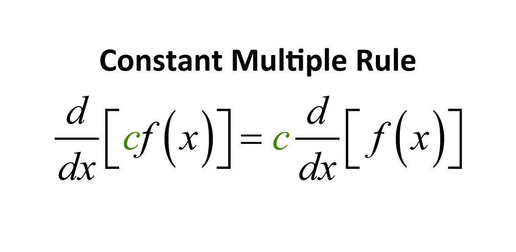
This diagram states the constant multiple rule in compact symbolic form, showing that $\frac{d}{dx}[c\cdot f(x)] = c\cdot f'(x)$ when $c$ is a constant. It emphasizes that the constant factor is carried unchanged into the derivative. The image aligns with the AP requirement to recognize that the derivative is $c\cdot f'(x)$ for differentiable functions multiplied by a constant. Source.

Key Characteristics and Interpretive Ideas

Understanding how the constant multiple rule affects a function’s graph and contextual meaning enriches a student’s ability to interpret derivatives beyond symbolic manipulation.

Graphical Interpretation

Multiplying a function by a constant vertically scales its graph:

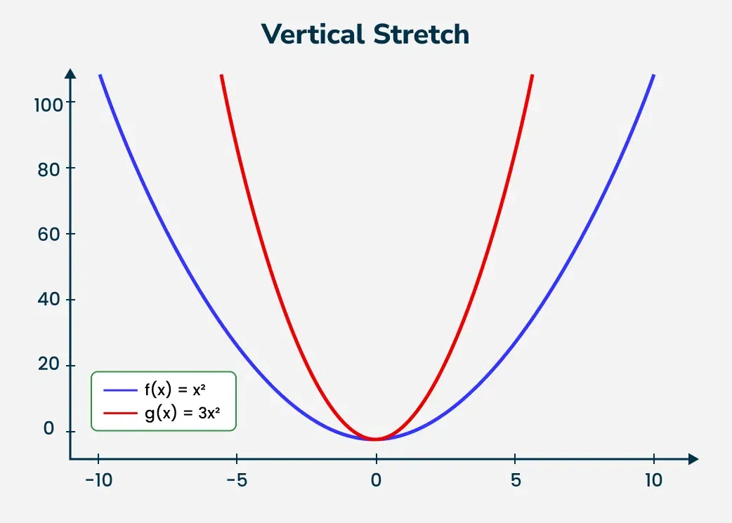
This graph compares the base function $f(x)=x^2$ with its vertically stretched version $g(x)=3x^2$. The red curve illustrates how multiplying by a constant increases steepness, scaling all slopes and therefore the derivative by the same factor. The visual focuses solely on vertical stretch, supporting conceptual understanding of the constant multiple rule. Source.

• If c>1, the graph stretches vertically, increasing all slopes proportionally.

• If 0<c<1, the graph compresses, decreasing the steepness of all slopes.

• If c<0, the graph reflects across the $x$-axis, reversing slope direction.

Because the derivative represents slope, each of these geometric effects directly influences $f'(x)$:

• Steeper graph → larger magnitude derivative

• Flatter graph → smaller magnitude derivative

• Reflection → opposite-signed derivative

These interpretations reinforce why the derivative of $c\cdot f(x)$ must be $c\cdot f'(x)$.

Contextual Interpretation

When applying the rule in real-world problems, constant multiples often represent scaling factors such as conversion units, pricing coefficients, or physical constants. The derivative then acquires a correspondingly scaled interpretation:

• If $f(x)$ models a quantity, $c\cdot f(x)$ may model cost, energy, or another scaled output.

• The derivative $c\cdot f'(x)$ then describes how quickly this scaled quantity changes with respect to the input variable.

This ensures consistency between the mathematical rule and its applied meaning.

Recognizing When the Rule Applies

Students must identify constants correctly to apply the rule efficiently. The rule applies only when:

• The multiplier is a constant, not a variable.

• The function being multiplied is differentiable.

• No additional structure (such as products or compositions) requires other derivative rules.

A constant may be:

• A real number (e.g., 5, –3, $\tfrac{1}{4}$)

• A symbolic constant (e.g., $k$, $C$)

• A physical constant (e.g., gravitational constant, growth factor)

If the multiplier involves $x$ or any expression that varies with $x$, then the constant multiple rule alone does not apply; instead, the product rule is required.

Strategic Use in Simplifying Derivatives

The constant multiple rule often appears in combination with other differentiation rules. It provides a first step in streamlining expressions before applying more advanced derivative techniques.

Students should adopt the habit of:

• Pulling out constant factors before differentiating.

• Separating complex expressions into manageable parts using sum and difference rules.

• Avoiding unnecessary algebra by recognizing when constants can simplify derivative steps.

This rule is particularly powerful when differentiating polynomials, trigonometric functions with coefficients, and exponential functions multiplied by real-number constants.

Practical Structure for Applying the Rule

To apply the constant multiple rule consistently, follow this layered approach:

• Identify any constant multipliers in the function.

• Confirm that the function multiplied by the constant is differentiable.

• Factor out the constant before taking the derivative.

• Differentiate the remaining function using the appropriate rule.

• Multiply the resulting derivative by the constant to obtain the final expression.

This structured method ensures clarity and reduces the likelihood of common mistakes such as differentiating the constant itself or incorrectly applying other derivative rules.

By mastering the constant multiple rule, students strengthen their foundational differentiation skill