Finding the equation of a tangent line is essential for understanding how derivatives describe local behavior, enabling precise linear approximations and meaningful interpretations of differentiable functions.

The Purpose of a Tangent Line

A tangent line provides the best linear prediction of a function’s value near a specific point. Because a differentiable function is locally linear, its behavior close to a chosen input can be modeled using a straight line. The tangent line captures both the instantaneous rate of change and the function’s value at a chosen point, making it a foundational tool for approximation and interpretation.

Understanding the Slope of a Tangent Line

The slope of the tangent line at a point is given by the function’s derivative at that point. When we compute a derivative, we are measuring how the dependent variable changes relative to the independent variable at a specific location on the curve.

This slope tells us whether the function is increasing or decreasing and how steeply it behaves near the point.

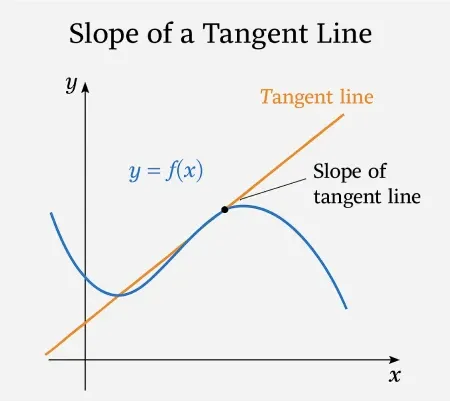
This graph shows a differentiable function $y=f(x)$ together with its tangent line at a point. The tangent line has the same slope as the curve at that point, illustrating the instantaneous rate of change. The labeled slope arrow reinforces that the derivative value represents the slope of this line. Source.

Before determining the full tangent line, it is necessary to know both the slope and a corresponding point on the curve. These two pieces of information uniquely determine a line.

General Form of a Tangent Line Equation

Once the slope and point are known, we use the point–slope form of a line. This structure emphasizes that the tangent line is anchored to the function at the chosen input value. In AP Calculus AB, this format is both standard and essential, especially when preparing linearizations for later use.

This representation ensures that the tangent line passes exactly through $(a,, f(a))$ and has slope $f'(a)$.

Essential Steps for Constructing a Tangent Line

Constructing a tangent line follows a clear and repeatable process. AP Calculus AB emphasizes understanding why each step matters as well as performing the computation accurately.

Step-by-Step Structure

Students should follow this sequence to ensure they identify all necessary components:

• Identify the point of tangency.
  Confirm the input value $a$ and compute $f(a)$ to anchor the line.

• Differentiate the function.
  Compute $f'(x)$ using standard derivative rules.

• Evaluate the derivative at the point.
  Substitute $x = a$ to obtain the slope $f'(a)$.

• Apply the point–slope form of a line.
  Construct the tangent equation using known values.

• Rewrite if needed for interpretation.
  Slope–intercept form may assist with graphical understanding, though point–slope form is typically preferred in calculus contexts.

Each step reinforces the connection between algebraic structure and the geometric meaning of derivatives.

Why Tangent Lines Matter in Context

A tangent line is more than an abstract construction; it conveys how a function behaves at a specific instant. Because the tangent line shares the function’s slope at one point, it indicates whether change is occurring rapidly, slowly, positively, or negatively. In applied settings, the tangent line can represent:

• A momentary trend in physical motion

• A brief snapshot of population change

• An economic model’s behavior at a specific production level

Although this subsubtopic does not delve into linearization, the tangent line is the basis for such approximations.

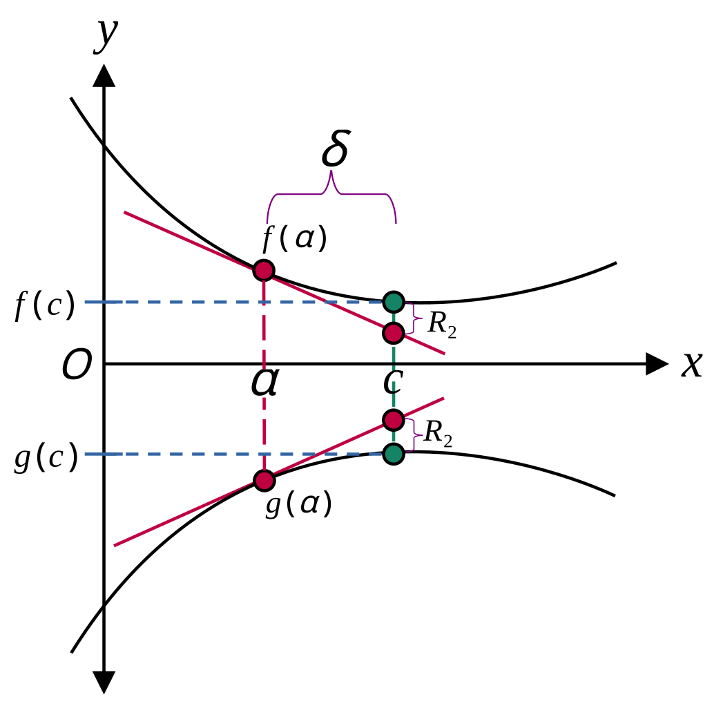
The figure shows two functions, $f$ and $g$, each with a tangent line drawn at the shared input $\alpha$, along with nearby points whose values are approximated by the tangent lines. It illustrates how a tangent line provides a local linear model for estimating function values near a point. The inclusion of symbols like $\delta$, $c$, and $R_2$ goes beyond AP requirements but merely marks distances and approximation errors. Source.

Understanding its form is fundamental for later topics such as estimating values, analyzing concavity effects on predictions, and interpreting real-world behaviors.

Notation and Interpretation

The tangent line’s slope is often written as $f'(a)$ or $\dfrac{dy}{dx}\big|_{x=a}$, both of which communicate an instantaneous rate of change. Students should interpret this slope in terms of:

• What quantity is changing

• The variable with respect to which it changes

• The units involved

Even though formal unit interpretation belongs to other subsubtopics, recognizing that the tangent line conveys a measurable rate strengthens comprehension of its purpose.

Communicating Tangent Line Results

A complete tangent line description must clearly identify:

• The function being considered

• The point of tangency

• The derivative calculation

• The final line written in a clear algebraic form

Clarity of communication is essential, especially when tangent lines are used to support arguments about function behavior or approximate values.

This structure ensures the tangent line serves as an accurate, meaningful linear model tied directly to the function’s instantaneous behavior.