AP Syllabus focus:
‘Understand that differentiable functions are locally linear, so when you zoom in near a point, the graph looks almost like a straight line that approximates the function.’
Local linearity describes how a differentiable function behaves extremely close to a point, where its graph appears nearly straight and can be approximated by a tangent line.
Understanding Local Linearity
A central idea in differential calculus is that differentiable functions are locally linear.

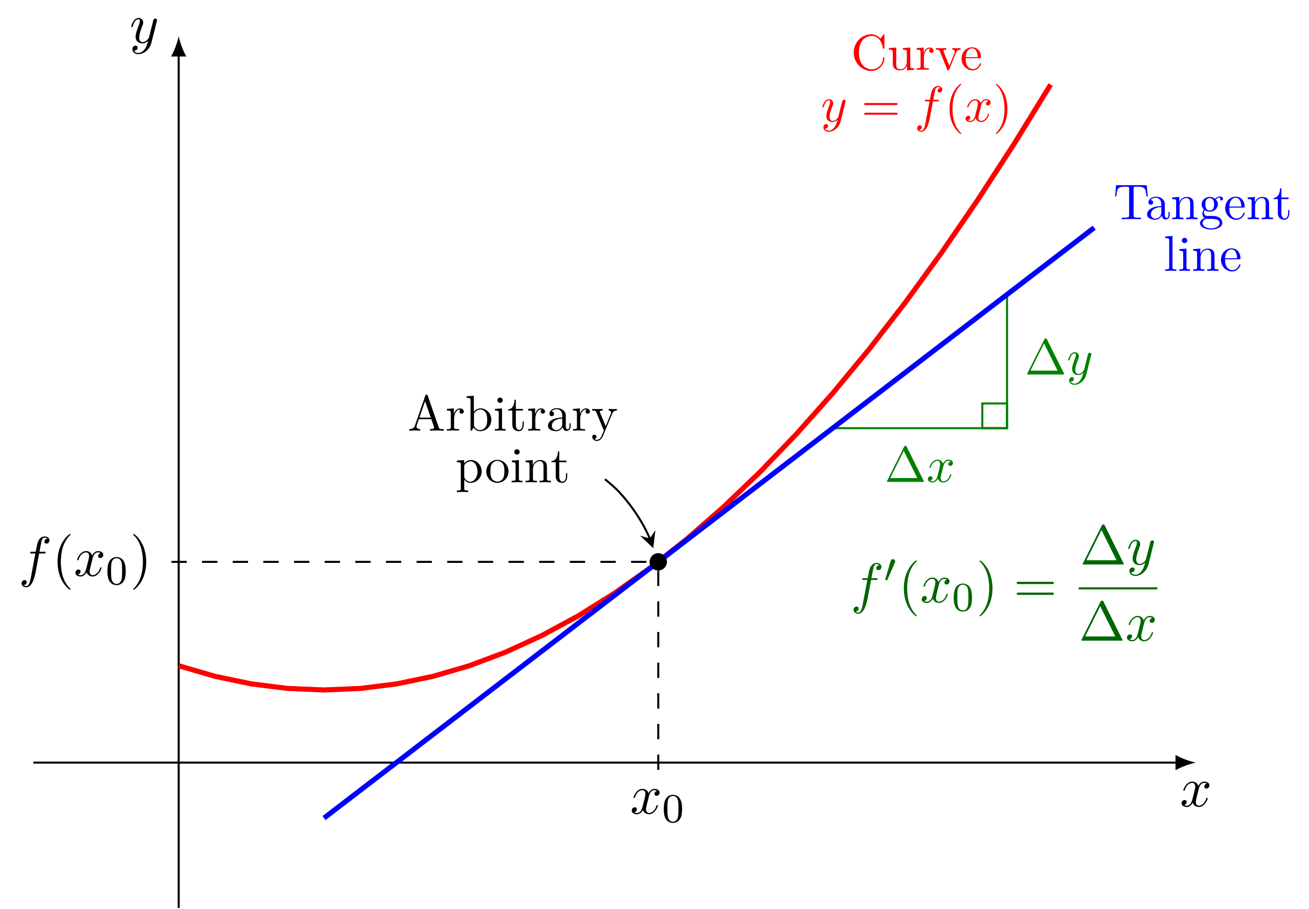
This diagram shows a smooth curve with a tangent line touching the graph at a single point. The tangent line illustrates how, near that point, the function behaves almost like a straight line with slope equal to the derivative. This visualization connects the abstract idea of to the concrete slope of a line that locally models the function. Source.
This means that if a function is differentiable at a point, then when you zoom in sufficiently close to that point, the curve becomes almost indistinguishable from a straight line. This straight line is the tangent line at that point, and it provides a powerful tool for approximating function behavior on small intervals surrounding the point of tangency.
When discussing local linearity, the foundational mathematical object is the derivative, which represents the slope of the tangent line at a specific input value. The derivative captures how fast the function changes at that exact moment, and local linearity relies on this feature to create accurate approximations.
Differentiability and Smoothness
A function must be differentiable at a point to exhibit local linearity. Differentiability ensures the function has no sharp corners, cusps, or discontinuities at that location.
Term: A function is differentiable at a point if its derivative exists at that point, meaning the function has a well-defined instantaneous rate of change there.
Because differentiability guarantees smoothness, the tangent line does more than simply touch the graph—it closely matches the function’s behavior in a small neighborhood. This idea is essential for concepts such as linearization and approximating values.
Between any two conceptual blocks, it is important to recognize that local linearity becomes more accurate the closer one moves to the point of tangency.
Zooming In on Curves
The phrase zooming in describes the graphical process of magnifying the area around a specific point on a curve. Each successive zoom level removes large-scale curvature, making the function appear flatter. Eventually, the curve resembles a straight line with slope equal to the derivative at that point.
When zooming in on differentiable functions, their curvature becomes negligible at sufficiently small scales. This property is what allows calculus students to treat complicated functions as simple linear ones in localized regions.
The Tangent Line as a Local Model
Because the graph looks increasingly linear, the tangent line serves as a local model for the function. The tangent line provides the best linear approximation to the function at that point.

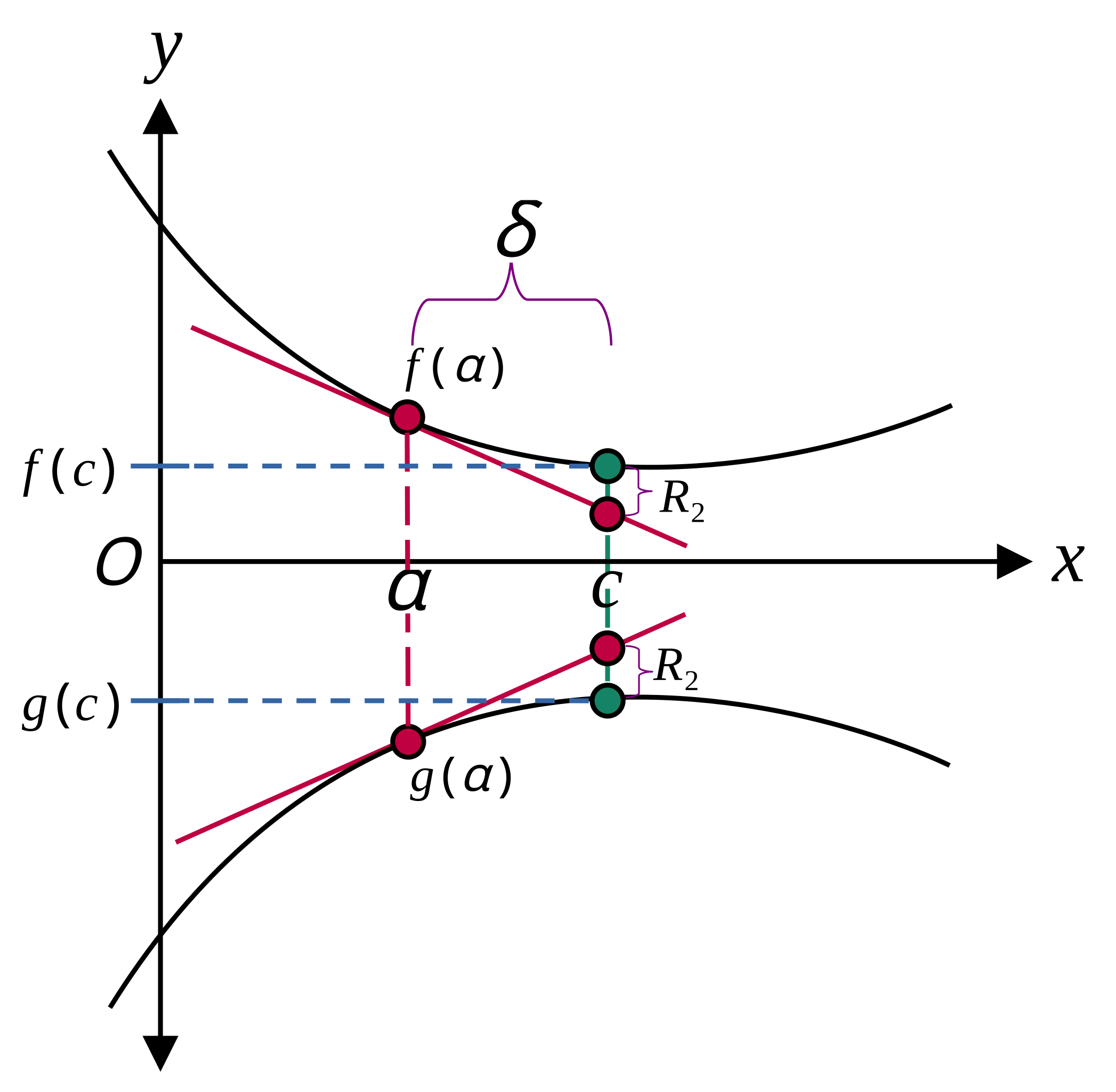
This figure shows two curves, and , each sharing a tangent line at the same point on the -axis. Near the tangency point, the tangent line closely matches the height of the curves, illustrating how can approximate for close to . The presence of two different functions emphasizes that local linear approximation is a structural idea applying broadly across many functions. Source.
= Function value at the point of tangency
= Derivative (slope) at the point of tangency
= Input variable representing a value near
= Center point where local linearity is applied
This equation is often called the point-slope form of the tangent line. It anchors the linear approximation process used later in linearization.
A crucial implication is that as approaches , the difference between the function and its tangent line becomes extremely small, demonstrating the practical accuracy of local linearity.
Why Local Linearity Matters
Local linearity provides the mathematical justification for approximating nonlinear behavior using linear functions. This is foundational for many applications in calculus and beyond.
Key reasons local linearity is important include:
It enables linearization, a method for estimating function values near a point.
It supports intuitive understanding of the derivative as a slope that not only touches but predicts nearby function behavior.
It provides the basis for advanced ideas in calculus, such as differentials and error estimation.
It allows students to simplify complex functions into manageable linear relationships when examining small-scale behavior.
Visual Interpretation
A deeper visual interpretation highlights the difference between the global shape of a curve and its local behavior. Globally, a curve may bend, oscillate, or change concavity. Locally, at a single point where the function is differentiable, the curve becomes almost indistinguishable from a straight line when viewed at a sufficiently fine scale. This reinforces the idea that the tangent line is not merely touching the curve—it is representing its instantaneous behavior.
Understanding this visual aspect helps students connect symbolic derivative expressions with the geometric meaning of slope and linearity.
Strengthening Conceptual Understanding
To solidify comprehension of local linearity, students should focus on the following ideas:
A differentiable function behaves like a straight line when examined very close to a point.
The derivative determines the slope of this locally linear behavior.
The tangent line is the simplest and most accurate model of the function near the point of tangency.
Local linearity is a property of differentiability and does not extend to points where the function is not smooth.
These conceptual points guide students in recognizing when linear approximations are appropriate and how they arise from foundational calculus principles.
FAQ
The interval must be small enough that the curve’s natural bend is negligible when compared with the slope at the point. This varies by function.
A practical test is to shrink the interval and observe whether the estimated values produced by the tangent line stabilise. If the approximation changes noticeably with smaller intervals, the scale is not yet sufficiently local.
Some differentiable functions have derivatives that change very rapidly, causing noticeable curvature even in small neighbourhoods.
Functions with steep concavity, oscillations or rapid variation in slope require extremely small intervals before the graph resembles a straight line.
Not exactly. Local linearity assumes the rate of change is approximately constant only within a very small interval.
Across larger intervals, the rate of change may vary significantly. The assumption is valid only in the immediate vicinity of the point of tangency.
Look for smoothness and gentle curvature near the point. Sharp bends or inflection points reduce the accuracy of linear behaviour.
A function that appears almost straight for a short horizontal stretch typically has strong local linearity, especially if the derivative does not change abruptly nearby.
Local linearity applies only when you can examine the function on both sides of the point.
At an endpoint, you can zoom in only from one side, so the notion still works but with reduced reliability. The tangent line may approximate the function on the available side, but the behaviour is less symmetric and more sensitive to boundary shape.
Practice Questions
(1–3 marks)
A differentiable function g has a graph that appears curved on a standard viewing window. When you zoom in closely near x = 2, the graph becomes nearly indistinguishable from a straight line with slope 5.
(a) State what this observation tells you about the local behaviour of g near x = 2.
(b) Estimate the value of g(2.1) using the idea of local linearity.
Question 1 (1–3 marks)
(a) 1 mark
• States that g behaves approximately like a straight line near x = 2 or that the tangent with slope 5 models the function locally.
(b) 1–2 marks
• Uses the idea that g(2.1) is approximately g(2) + 5(0.1). (1 mark)
• Writes a correct numerical expression or gives a correct numerical estimate. (1 mark)
(Allow use of g(2) as an unspecified constant if not given; method marks available.)
Total: 3 marks
(4–6 marks)
A function f is differentiable for all real numbers. At x = 4, the function satisfies f(4) = 7 and f ’(4) = −3.
(a) Explain how the concept of local linearity justifies using a tangent line to approximate f near x = 4.
(b) Write the equation of the tangent line to f at x = 4.
(c) Use your tangent line to approximate f(3.8).
(d) Give one reason why this approximation might differ from the actual value of f(3.8).
Question 2 (4–6 marks)
(a) 1–2 marks
• States that differentiability implies the graph appears linear when viewed sufficiently close to x = 4. (1 mark)
• States that the tangent line gives the best linear approximation to the function near that point. (1 mark)
(b) 1 mark
• Writes the equation of the tangent line: y = 7 − 3(x − 4) or equivalent simplified form.
(c) 1–2 marks
• Substitutes x = 3.8 into the tangent line. (1 mark)
• Gives the correct numerical approximation. (1 mark)
(d) 1 mark
• Gives a valid reason, such as the function not being perfectly linear, curvature of the graph near x = 4, or limitations of local approximation when moving away from the tangency point.
Total: 6 marks

