Linearization provides a powerful way to approximate complex function values using the tangent line, allowing students to estimate outputs quickly when exact computation is inefficient.

Understanding Linearization in Context

The idea of linearization centers on the fact that differentiable functions behave almost like straight lines when viewed very close to a specific point. This local straight-line behavior enables us to replace a curved function with its tangent line, which is easier to compute and manipulate.

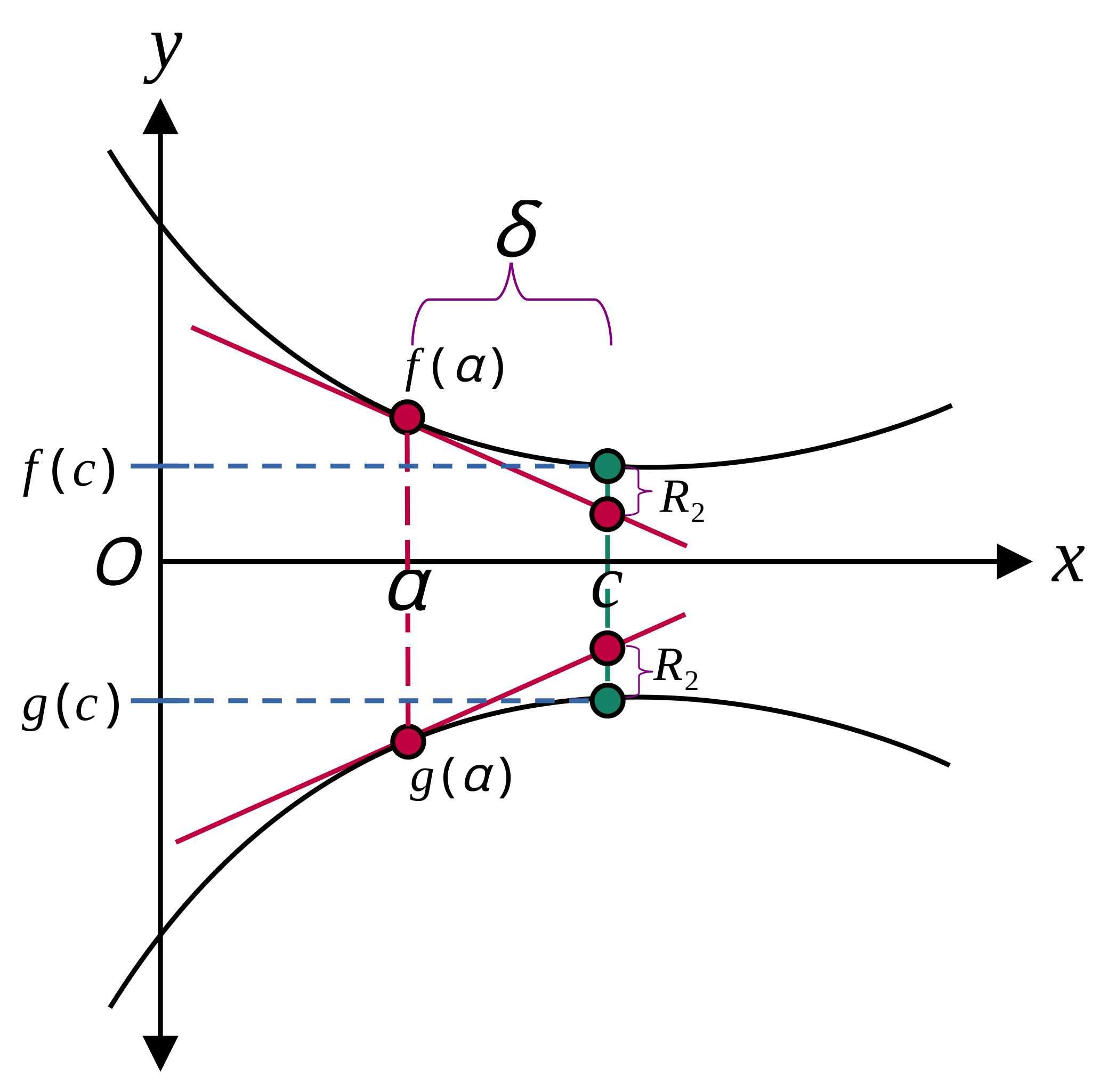
This diagram shows two differentiable curves alongside their tangent lines, illustrating how each tangent line provides a local linear approximation. Near the point of tangency, the line and curve nearly overlap, demonstrating the principle of linearization. Source.

When studying linearization, the essential task is to connect the behavior of a function to the behavior of its tangent line. The tangent line acts as a local linear model, capturing the function’s instantaneous rate of change and using that information to estimate new values.

Constructing a Linearization

To create a linearization, one identifies a function that is differentiable at a chosen point and computes both the function value and its derivative at that point. These quantities define the tangent line, which becomes the approximating linear function. Because the tangent line shares the same slope and value as the function at that point, the approximation is typically strongest for values of the input variable very close to the chosen point.

Key Components of a Tangent Line Approximation

A tangent line approximation depends on two essential pieces of information: the value of the function at the point of tangency and the value of the derivative at that same point. These establish the height and steepness of the tangent line. After determining these values, one forms an expression that mimics the nearby behavior of the original function.

This expression models the function’s behavior around $x = a$. After forming the linearization, students can substitute a nearby input into $L(x)$ to approximate the function’s value.

Why Linearization Works

Because differentiable functions are locally linear, their tangent lines provide close approximations when zoomed in sufficiently near the point of tangency. This closeness occurs because the derivative captures how the function changes instantly at that point. When $x$ is close to $a$, the difference between the actual curve and the tangent line becomes small enough that the linear model offers a robust estimate of the true value.

Interpreting Linearization Results

Interpreting the meaning of a linear approximation requires relating the tangent line values back to the context of the function. Since the linearization reflects how the function behaves around a particular input, the result represents an estimate of the original quantity at a nearby point. This estimate should always be read with attention to the function’s context, noting what is being approximated and the relevant units.

When using linearization, it is essential to consider whether the tangent line lies above or below the actual function near the point of tangency. This depends on the function’s concavity, which indicates whether the approximation might slightly overestimate or underestimate the true value. Although determining concavity formally belongs to another subtopic, understanding that curvature affects accuracy helps students evaluate their approximations thoughtfully.

Process for Using Linearization to Approximate Values

Students can rely on the following structured approach:

• Identify the function and select the point $a$ where the value and derivative can be easily computed.

• Evaluate the function at $a$ to determine $f(a)$.

• Differentiate the function and compute the derivative value $f'(a)$.

• Construct the linearization using the expression $L(x) = f(a) + f'(a)(x - a)$.

• Substitute the nearby input into the linearization to approximate the function’s value.

• Interpret the result in context, ensuring that units and meaning align with the original function.

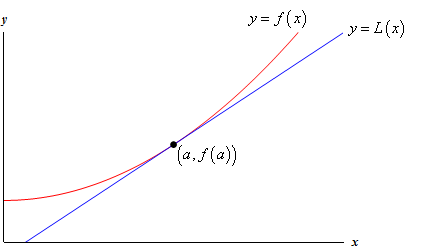
This graph depicts the function $f(x)=\sqrt[3]{x}$ together with its tangent line at $x=8$, illustrating how a linearization estimates nearby function values. Close to the point of tangency, the line and curve align closely, demonstrating accuracy; farther away, the approximation becomes less reliable. The specificity of the example exceeds general syllabus requirements but clearly shows the behavior of linear approximations. Source.

Approaching linearization with this sequential process helps ensure clarity, precision, and strong alignment with the AP Calculus AB expectations.