Price elasticity of supply explains how strongly producers adjust output when market price changes. This page focuses on the real-world conditions that make supply more or less responsive, especially input alternatives and production flexibility.

Core idea: responsiveness on the producer side

Elasticity of supply is about how easily firms can change quantity supplied when the good’s own price changes. The key determinants all operate through one question: how quickly and cheaply can producers expand (or contract) output without sharply increasing marginal cost?

Price elasticity of supply (PES)

PES is unit-free and depends on production constraints, available technology, and input markets, not simply on the slope of a supply curve drawn on a graph.

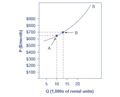
Supply curve for apartment rentals with two price–quantity points used to compute price elasticity of supply (PES). The dashed guides emphasize the changes in $P$ and $Q_s$ that feed into the percent-change formula. This visual helps distinguish “elasticity” (a ratio of percentage changes) from the geometric slope of the curve. Source

What determines elasticity of supply?

1) Time horizon (immediate, short run, long run)

Time is often the dominant determinant of PES because more time allows more adjustment margins.

• Immediate/very short run: Supply tends to be inelastic.

  • Firms are stuck with current capacity, staffing, and inventories.

• Short run: Supply becomes more elastic as firms can:

  • add shifts, pay overtime, reorder materials, intensify use of existing capital

• Long run: Supply is typically more elastic because firms can:

  • build new plants, adopt new processes, enter/exit the industry, redesign products

2) Availability and price of alternative inputs (syllabus emphasis)

Producers combine inputs (labour, capital, raw materials, components).

Supply is more elastic when firms can switch among inputs without large cost increases.

• If the price of alternative inputs is low (or falling), firms can expand output more easily because:

  • they can substitute toward relatively cheaper inputs

  • marginal cost rises more slowly as production increases

• If the price of alternative inputs is high (or rising), supply is less elastic because:

  • scaling up requires expensive substitutions or bidding inputs away from other uses

  • marginal cost rises quickly, limiting responsiveness

This determinant is especially important when a key input is scarce or has few close substitutes (for example, a specialised component or location-specific resource).

3) Spare capacity and ability to vary utilisation

Spare capacity makes it easier to expand output when price rises.

• More spare capacity → more elastic supply

  • idle machines, underused retail space, unused trucking capacity

• Operating near full capacity → less elastic supply

  • expansion requires costly investment, maintenance delays, or congestion

4) Input mobility and factor specificity

Supply is more elastic when inputs can move into the industry quickly.

• High mobility (generic labour skills, widely available materials) → higher PES

• Specific factors (highly specialised labour, custom capital, unique land) → lower PES

• Barriers such as licensing, training time, or geographic immobility reduce responsiveness.

5) Inventories and storability

If output can be stored and inventory exists, firms can respond more to price changes.

• Large inventories/low storage cost → more elastic (release stock when price rises)

• Perishability or expensive storage → less elastic

• For many services, storage is impossible, which tends to reduce short-run elasticity.

6) Ease of scaling production and technological flexibility

Technology shapes how quickly marginal cost increases as output expands.

• Flexible production processes (modular equipment, scalable software, standardised components) → higher PES

• Rigid processes (fixed-proportion technologies, long setup times, bottleneck stages) → lower PES

• Learning-by-doing and process innovation can increase PES over time by lowering adjustment costs.

7) Institutional and contractual constraints

Even when technically feasible, firms may be constrained by rules and agreements.

• Long-term input contracts, union work rules, or scheduling constraints can reduce elasticity.

• Regulations (permits, environmental compliance timelines) can slow expansion, lowering PES.

• Conversely, streamlined permitting or flexible contracting can raise PES.

Common AP-level interpretations

Reading determinants without calculation

When asked to justify “more elastic” vs “more inelastic” supply, tie your reasoning to one or more of these mechanisms:

• adjustment speed (time)

• availability/cost of substitutable inputs (including the price of alternative inputs)

• capacity limits

• mobility of resources

• inventory/storage feasibility

• regulatory/contractual limits