
AP Syllabus focus:
‘Detailed explanation on calculating the slope, b, of the regression line using the formula: b = r(sy/sx), where r is the correlation coefficient between x and y, sy is the sample standard deviation of the response variable y, and sx is the sample standard deviation of the explanatory variable x. The section will highlight the importance of understanding the slope's role in the regression model.’
This section develops a clear understanding of how to compute the slope of a least-squares regression line and why this value is essential for interpreting linear relationships in bivariate quantitative data.
Calculating the Slope of the Regression Line
The slope of the least-squares regression line is a foundational element of linear modeling, describing how predicted values of the response variable change relative to the explanatory variable. In AP Statistics, emphasis is placed not only on computing the slope but also on recognizing its conceptual meaning within real-world data contexts.
Understanding the Role of the Slope
The slope indicates the predicted change in the response variable for a one-unit increase in the explanatory variable. When analyzing two quantitative variables, recognizing this rate of change helps clarify both the direction and magnitude of their linear association. The slope integrates information from the distribution of each variable and from the correlation coefficient, enabling a standardized and statistically justified measure of association.
Slope of the Regression Line (b): The amount by which the predicted response variable changes, on average, for each one-unit increase in the explanatory variable.
Because the least-squares regression line minimizes the squared residuals, its slope is not arbitrary; it is systematically determined using sample statistics that reflect the strength of linear association and the spread of each variable.
Components Required for Calculating the Slope
To compute the slope, AP Statistics uses a formula that incorporates three essential components:
Correlation coefficient (r): Measures the strength and direction of the linear association.
Standard deviation of y (sy): Represents the spread of the response variable.
Standard deviation of x (sx): Represents the spread of the explanatory variable.
These components ensure the slope reflects both the variability within each variable and the degree to which the variables move together.
The Slope Formula
EQUATION
= Correlation coefficient measuring strength and direction of linear association
= Standard deviation of the response variable (y)
= Standard deviation of the explanatory variable (x)
This equation highlights that the slope increases in magnitude when the correlation becomes stronger or when the response variable varies more relative to the explanatory variable. It also ensures that the sign of the slope matches the sign of the correlation: a positive correlation yields a positive slope, and a negative correlation yields a negative slope.
The formula serves as a bridge between descriptive statistics (standard deviations and correlation) and inferential modeling (linear regression), reinforcing the idea that a regression line is statistically determined and not simply visually estimated.
You can visualize the slope as how steep the regression line is when plotting the response variable against the explanatory variable.
Interpreting the Slope in Context
Understanding the slope requires more than being able to compute it numerically. Students must also interpret the slope meaningfully within the scenario being analyzed. Because the slope describes average predicted change, its interpretation always includes:
Direction:
A positive slope indicates that larger x-values are associated with larger predicted y-values.
A negative slope indicates that larger x-values are associated with smaller predicted y-values.
Rate of change:
The numerical value quantifies how rapidly the response is expected to change.
Units: The slope’s units come from the ratio of the units of y to the units of x, reinforcing its interpretation as a rate.
Such interpretations must rely on the context of the data and the meaning of the variables.
In a simple linear regression model, the least-squares regression line has the form ŷ = a + bx, where b is the slope and a is the y-intercept.
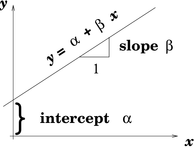
A labeled regression line showing the intercept and slope, reinforcing the structure of the equation ŷ = a + bx and the geometric meaning of each coefficient. Source.
Why the Slope Matters in Least-Squares Regression
The slope plays a critical role in the least-squares regression model for several reasons:
It determines how the regression line tilts across the scatterplot and thus shapes all predictions.
It reflects the influence of variability in both variables, ensuring predictions are appropriately scaled.
It encodes the sign and magnitude of the linear relationship, making it indispensable for describing the association.
If r is positive, then b is positive and the regression line slopes upward; if r is negative, b is negative and the line slopes downward, and when r is near zero the line is nearly flat.
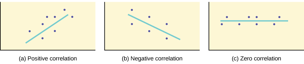
Three scatterplots showing positive, negative, and near-zero slope, illustrating how the correlation r determines the direction and steepness of the regression slope. Source.
Key Points for AP Statistics Students
Linear regression relies on quantitative variables only. Understanding the slope is inseparable from understanding linear relationships.
Slope must always be interpreted in context. Even when computed correctly, a slope without context cannot provide meaningful insight.
The slope formula connects correlation with prediction. Students should recognize that the regression slope emerges from measurable characteristics of the sample, not subjective judgment.
The slope’s sign and magnitude reflect the data’s structure. This reinforces the importance of examining scatterplots before and after computing regression components.
By mastering the computation and interpretation of the slope using , students gain essential tools for analyzing and explaining linear relationships within bivariate data—an integral skill across AP Statistics.
FAQ
The slope uses the ratio of the standard deviations of y and x, which adjusts for the units and spread of each variable. This prevents the slope from being distorted when variables are measured on very different scales.
Because the formula incorporates correlation, which is unitless, the resulting slope reflects the true strength and direction of association rather than the measurement units themselves.
If x is multiplied by a constant, the slope is divided by the same constant. This is because increasing the unit size reduces the number of units per observed change.
Importantly, the correlation does not change when rescaling occurs, so only the slope is affected, not the strength of the linear association.
Slope depends on both correlation and the ratio of standard deviations. Two data sets may share the same r but have different spreads in x or y.
This means that identical linear association strength can still produce very different predicted changes depending on how variable each variable is.
Outliers in x affect both the correlation and the standard deviation of x, which directly influences the slope.
High-leverage points can disproportionately affect the tilt of the regression line, making the slope steeper or flatter than it would be based on the central mass of the data.
Yes, if different variables are designated as explanatory and response. Regression of y on x and x on y produces lines with different slopes because each minimises residuals in a different direction.
This highlights why identifying the appropriate explanatory variable is essential before calculating and interpreting the slope.
Practice Questions
Question 1 (1–3 marks)
A researcher finds that the correlation between the number of hours studied (x) and an exam score (y) is 0.72. The standard deviation of exam scores is 12, and the standard deviation of study hours is 4.
(a) Calculate the slope of the least-squares regression line used to predict exam score from hours studied.
(b) Interpret the slope in context.
Question 1 (1–3 marks)
(a) 2 marks
• Correct method: b = r(sy / sx). (1 mark)
• Correct numerical slope of 2.16 (accept answers rounded to 2.2). (1 mark)
(b) 1 mark
• Correct contextual interpretation: For each additional hour studied, the predicted exam score increases by about 2.16 points. (1 mark)
Question 2 (4–6 marks)
A biologist records the body length (x, in centimetres) and running speed (y, in metres per second) of a sample of 12 lizards. The correlation between length and speed is -0.41. The standard deviation of speed is 0.9, and the standard deviation of length is 3.1.
(a) Calculate the slope of the least-squares regression line for predicting running speed from body length.
(b) Explain what the sign and magnitude of this slope indicate about the relationship between length and speed.
(c) Discuss whether the slope alone is sufficient to judge how well body length predicts running speed, giving one additional measure or piece of information that would be useful.
Question 2 (4–6 marks)
(a) 2 marks
• Correct method using b = r(sy / sx). (1 mark)
• Correct numerical slope of approximately -0.12 (accept answers around -0.119). (1 mark)
(b) 2 marks
• States that the negative sign indicates that longer lizards tend to have lower predicted running speeds. (1 mark)
• Notes that the slope is relatively small in magnitude, indicating that the rate of decrease in predicted speed per centimetre of length is modest. (1 mark)
(c) 2 marks
• States that the slope alone does not describe the strength of prediction. (1 mark)
• Identifies an additional useful measure or information, such as the correlation coefficient, the coefficient of determination, or examination of a scatterplot. (1 mark)
