When a transformation is used to improve linearity, the next step is deciding whether the new model is actually better. AP Statistics emphasizes residual plots and $r^2$ as the main evidence.

What makes a transformed model better

A transformed regression model should be judged by how well it supports prediction, not just by whether it looks different from the original model.

A better model usually does two things:

• it leaves less visible structure in the residuals

• it explains more of the variation in the response

The specification gives two signals of improvement: a more random residual plot and an $r^2$ value closer to 1. The word can matters. Either feature may suggest improvement, but neither should be treated as automatic proof on its own.

Residual plots: the most direct check

A residual plot is often the clearest way to tell whether a transformation helped. After transformation, the residuals should look more like random scatter around 0.

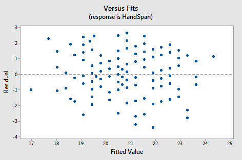
Residuals versus fitted values for a straight-line regression with the residuals scattered randomly around 0 and roughly constant vertical spread. This is the visual pattern you want when a linear model (or a transformed linear model) is appropriate for prediction. Source

What to look for

In a better transformed model, the residual plot should show:

• no obvious curve

• no clear increasing or decreasing pattern

• no funnel shape or changing spread

• points scattered fairly evenly above and below 0

A plot that becomes more random after transformation suggests the linear model is matching the data more appropriately. That matters for prediction because systematic leftover patterns mean the model is still missing structure.

The comparison is relative.

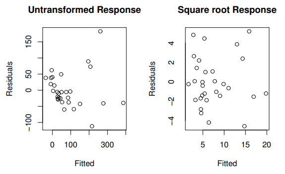
Residual-fitted plots shown before and after a square-root transformation of the response: the untransformed plot shows changing spread, while the transformed plot has more uniform scatter. This illustrates how a transformation can improve the model form for prediction by making residual behavior closer to random noise. Source

You are not asking whether the transformed residual plot is perfect; you are asking whether it is more random than before. If the original model showed curvature and the transformed model removes most of that pattern, the transformation likely improved the model. If strong structure remains, the transformation did not fully solve the problem.

Why randomness matters

Prediction works best when the unexplained part of the model behaves like random noise instead of following a pattern. A nonrandom residual plot suggests that the model is still missing some feature of the relationship. That missing feature can make predictions less dependable, especially across different parts of the data set.

Because of this, a transformed model with a noticeably more random residual plot is often preferred even before looking at any numerical summary. The residual plot directly shows whether the model form has improved.

Using $r^2$ as supporting evidence

The second clue is whether $r^2$ moves closer to 1 after transformation.

Diagram illustrating $r^2$ (coefficient of determination) as a comparison of explained variation versus unexplained variation in a linear regression. The colored areas help connect the numeric value of $r^2$ to the idea of “how much variability the model accounts for,” which is why larger $r^2$ can support (but not replace) residual-plot evidence. Source

A larger $r^2$ means the model accounts for more of the variation in the response. In AP Statistics language, that suggests the transformed model gives a stronger linear fit.

However, a higher $r^2$ should be treated as supporting evidence, not the only evidence. A model can have a fairly large $r^2$ and still show a patterned residual plot. In that case, prediction is less trustworthy because the model is not fully capturing the form of the relationship.

Small differences in $r^2$ should also be interpreted carefully. If one transformation raises $r^2$ only slightly but makes the residual plot much more random, the improvement in residual behavior is usually the more important sign.

Comparing models for prediction

When comparing an original model with a transformed model, use both pieces of information together.

Strong evidence of improvement

You have the strongest case for the transformed model when:

• the residual plot is noticeably more random

• the residuals show less pattern or changing spread

• $r^2$ is closer to 1 than before

If both criteria improve, you can reasonably say the transformed model is better for prediction.

Mixed evidence

Sometimes the evidence is mixed. A transformed model may have a more random residual plot but only a small change in $r^2$. In that situation, focus on whether the transformation reduced nonrandom structure, because prediction depends on the model form being appropriate.

If $r^2$ increases but the residual plot still shows a clear pattern, be cautious. The transformation may have strengthened the numerical fit without fixing the model form well enough for reliable prediction.

How to describe this on an AP Statistics response

A clear evaluation should directly compare the two models and link the evidence to prediction.

Useful language

• “The transformed model appears better because the residual plot is more random, with no clear pattern.”

• “Its $r^2$ is closer to 1, so the model explains more of the variation in the response.”

• “Because the residuals show less structure, the transformed model is more appropriate for prediction.”

Avoid statements such as “the transformation definitely makes the model correct” or “a higher $r^2$ always means the better model.” The AP standard is more careful: these features indicate a better transformed regression model, especially when they are considered together.