
AP Syllabus focus:
‘Discuss probabilistic reasoning as a foundation for anticipating patterns in data. Explain how probability distributions, including the binomial distribution, can be constructed using rules of probability or estimated through simulations with random number generators. This approach allows for understanding how distributions represent probabilities of outcomes in a quantifiable manner.’
Probability distributions provide a structured way to describe how likely different outcomes are in random processes, helping statisticians model uncertainty and anticipate long-run patterns in data.
Constructing Probability Distributions
Understanding how to construct probability distributions is essential for interpreting and predicting outcomes in statistical settings. A probability distribution assigns a probability to each possible value of a random variable, making it a fundamental tool for analyzing random behavior.
Foundations of Probabilistic Reasoning
Probabilistic reasoning relies on recognizing that random processes exhibit variability, but this variability follows predictable long-run patterns. Constructing probability distributions requires identifying all possible outcomes, determining how likely each outcome is, and organizing these probabilities in a clear, quantitative structure.
Random Processes and Their Role in Distributions
A random process is a situation in which outcomes are determined by chance. Because each outcome is unpredictable in the short run but follows stable relative frequencies over many repetitions, random processes form the basis for meaningful probability distributions. By viewing data generation as the result of repeated random processes, probability distributions help quantify the likelihood of various outcomes occurring.
Steps in Constructing a Probability Distribution
When building a probability distribution, the process typically involves the following key components:
Identifying the random variable: Determine the numerical quantity of interest produced by the random process.
Listing all possible outcomes: Specify each distinct value the random variable can assume.
Assigning probabilities: Use rules of probability or simulations to quantify the likelihood of each outcome.
Ensuring validity: Check that every probability is between 0 and 1 and that all probabilities sum to 1.
This structured approach ensures that the distribution accurately represents the underlying random behavior.
Using Rules of Probability to Construct Distributions
Rules of probability serve as a mathematical foundation for determining the likelihood of outcomes. These rules allow distributions to be derived analytically. Key rules include:
The sum of all outcome probabilities must equal 1.
The probability of any event is the sum of the probabilities of the outcomes it contains.
Probabilities must reflect the nature of the random process, such as independence, the number of trials, or success–failure structure in binomial settings.
Analytically constructed distributions provide exact probabilities and are essential in formal statistical modeling.
For a discrete random variable, a bar chart or probability histogram displays each possible value on the horizontal axis and its probability on the vertical axis.
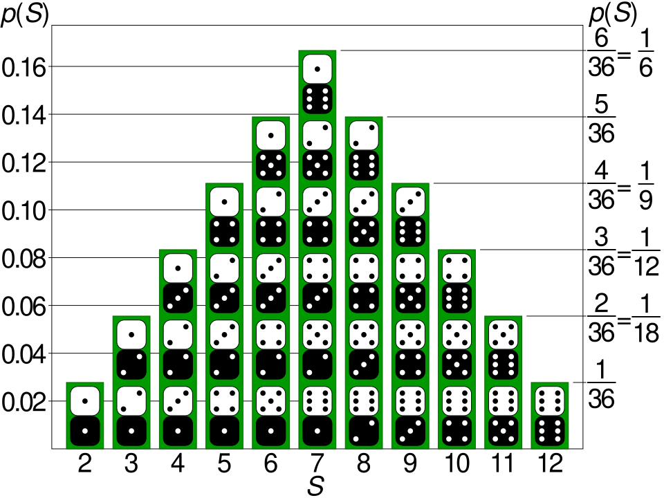
This bar chart displays the probability distribution for the sum of two fair dice, with bars representing the likelihood of totals from 2 to 12 and the highest bar at 7 where the most combinations occur. Source.
Constructing Distributions Through Simulation
Simulation is a powerful method for building probability distributions when theoretical calculation is difficult or when students need to visualize long-run behavior. A simulation models a random process using repeated, computer-generated or manually generated trials.
Simulations typically involve:
Representing outcomes using random number generators.
Conducting a large number of simulated trials.
Counting frequencies of outcomes.
Converting frequencies to relative frequencies, which serve as estimated probabilities.
By generating many trials, simulations approximate the true probability distribution, demonstrating how probabilities emerge from repeated random behavior.
The Role of Random Number Generators
Random number generators (RNGs) provide a reproducible and unbiased way to simulate random outcomes. They allow learners to mimic the randomness inherent in real-world processes while efficiently producing large datasets. These simulated datasets help approximate probability distributions when theoretical approaches are impractical or when exploring new concepts like the binomial distribution.
Probability Distributions as Representations of Outcome Likelihoods
A probability distribution summarizes the likelihood of all possible outcomes of a random variable. By organizing probabilities systematically, distributions allow students to understand which outcomes are typical, which are unusual, and how likely each scenario is. This quantitative summary is central to predicting patterns in data.
Constructing the Binomial Distribution
The construction of the binomial distribution is an important application of probability rules and simulation. Although detailed formulas are addressed in later subsubtopics, this section emphasizes how binomial distributions arise from:
Repeated independent trials
Only two possible outcomes per trial
A constant probability of success
The counting of successes across all trials
A binomial distribution can be created analytically using rules of probability or empirically through simulation. Both approaches reinforce the idea that distributions describe the quantified likelihood of each possible number of successes.
In practice, simulated distributions based on many trials can closely mimic the theoretical distribution obtained from probability rules.
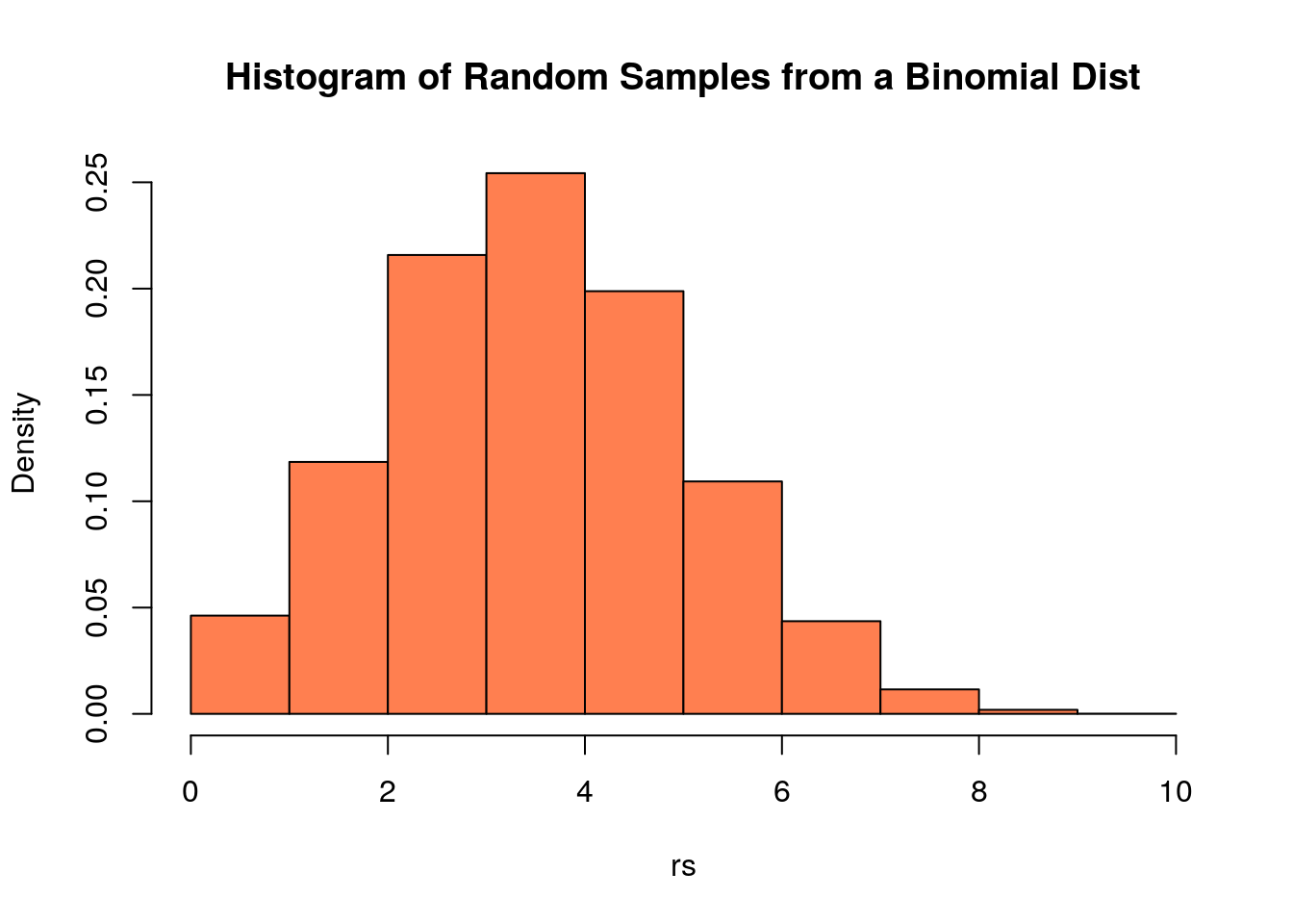
This histogram shows 10,000 simulated observations from a binomial distribution, with bar heights representing relative frequencies that approximate the distribution’s true theoretical shape. Source.
Importance of Constructing Probability Distributions
Constructing probability distributions helps students move from intuitive reasoning about chance to formal, quantitative analysis. By using rules of probability or simulations, students gain insight into how patterns emerge in repeated trials and why probability models are essential for understanding randomness in data.
FAQ
A frequency distribution summarises how often outcomes occur in observed data, while a probability distribution describes how likely outcomes are expected to occur in a random process.
A probability distribution does not require collected data; it can be theoretical or simulated.
A frequency distribution becomes a probability distribution only when frequencies are converted into proportions that sum to 1.
A probability distribution is valid only if all listed probabilities meet two conditions:
• Every probability is between 0 and 1.
• The total of all probabilities equals 1.
A quick check involves summing the probabilities and confirming there are no negative values or values exceeding 1. Any violation means the distribution is not properly constructed.
With more simulated trials, the relative frequencies of outcomes become more stable. This means the distribution increasingly reflects the true long-run behaviour of the random process.
Larger simulation sizes also reduce the influence of random fluctuations, smoothing out irregularities that occur in small samples.
Simulations allow comparison between expected behaviour and empirical results under controlled conditions.
If the simulated distribution consistently diverges from the theoretical one, possible issues include:
• Incorrect assumptions about independence or outcome likelihood
• Misidentified random variables
• Coding or procedural errors in the simulation itself
The set should include every distinct outcome that the random variable can take, without combining categories unless theoretically justified.
Too few categories can hide important structure, while too many can make the distribution unnecessarily complex. The key is matching the level of detail to the purpose of the analysis and the nature of the random process.
Practice Questions
Question 1 (1–3 marks)
A factory tests a machine that randomly produces items classified as either acceptable or defective. During a long simulation run, the relative frequency of acceptable items stabilises at 0.92.
a) Identify the random variable in this context. (1 mark)
b) State the probability distribution value associated with producing an acceptable item. (1 mark)
Question 1
a) 1 mark: Correctly identifies the random variable as the number or classification of items produced (acceptable or defective).
Award the mark for: “The random variable is the classification of an item: acceptable or defective,” or equivalent.
b) 1 mark: States the probability of producing an acceptable item as 0.92.
Accept any phrasing that clearly identifies 0.92 as the probability.
Question 2 (4–6 marks)
A student uses a random number generator to simulate the number of successful free throws a basketball player makes in 15 attempts. Each simulation run counts the number of successes and records it. The student repeats the entire simulation process 10 000 times and constructs a probability distribution for the number of successful free throws.
a) Explain why a simulation is appropriate for constructing this distribution. (2 marks)
b) Describe the steps required to construct the probability distribution from the simulation results. (3 marks)
c) State one advantage of using simulation instead of calculating the distribution analytically. (1 mark)
Question 2
a) 2 marks:
1 mark for stating that the process involves chance and repeated trials, making simulation appropriate.
1 mark for noting that simulation approximates the long-run relative frequencies when theoretical calculation is difficult or time-consuming.
b) 3 marks:
1 mark for describing identification of the random variable (number of successful free throws).
1 mark for explaining the need to run many simulated trials and record outcomes.
1 mark for converting outcome frequencies into relative frequencies to form the probability distribution.
c) 1 mark:
Any valid advantage, such as: simulations provide an empirical approximation without requiring complex calculations; simulations help visualise long-run behaviour; simulations can model conditions too complex for analytical methods.
