
AP Syllabus focus:
‘Outline the effects of linear transformations on random variables, specifically the transformation of a random variable X into Y using a linear equation Y = aX + b. Describe how such transformations affect the probability distribution, mean, and standard deviation of random variables, noting that the transformation maintains the shape of the distribution and how the parameters (mean and standard deviation) are adjusted.’
Linear transformations allow statisticians to rescale or shift a random variable without changing its fundamental shape, making them essential for interpreting and comparing probability distributions in meaningful ways.
Understanding Linear Transformations
A linear transformation applies a rule of the form to a random variable X, where a and b are real numbers. This process creates a new random variable Y whose values depend directly on the values of X. Linear transformations are widely used to convert units, adjust scales, or re-express data.
Linear Transformation: A rule that maps a random variable to a new variable through the equation , where and are constants.
One key property of linear transformations is that they preserve the shape of the probability distribution. Whether the distribution is symmetric, skewed, uniform, or discrete, applying does not alter its form. Only its location and spread change.
Effects on the Probability Distribution
While the shape is unchanged, the location and scale of the probability distribution shift in predictable ways. These changes occur because the transformation modifies the outcomes of the random variable without altering their relative likelihoods. Students should recognize that the transformation affects:
The center of the distribution
The spread, depending on the value of a
The orientation, if a is negative
The units and interpretation of outcomes
The preservation of shape means, for example, that a distribution that is right-skewed before transformation remains right-skewed afterward.
The transformation rescales the variable, and the units of measurement change, which can alter the interpretation of average outcomes and variability.
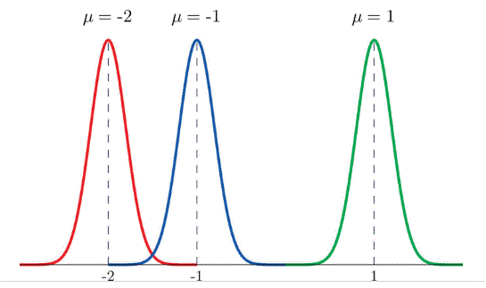
This figure shows how adding a constant shifts a distribution left or right without changing its overall shape or spread. Source.
Effects on the Mean
Linear transformations directly affect the mean, also known as the expected value, of the random variable. The transformation shifts and scales the center according to the constants a and b.
EQUATION
= Mean of transformed variable
= Mean of original variable
= Multiplicative scaling constant
= Additive shift constant
Because the mean reflects an average outcome, multiplying all outcomes by a scales the mean, while adding b shifts it. These changes help contextualize the transformed variable in new units or scales, which is particularly important when interpreting statistical output.
A sentence explaining impact: When a transformation is applied, the resulting mean reflects how both scaling and shifting modify the central location of the distribution.
Effects on the Standard Deviation
The standard deviation measures the variability of a random variable, and linear transformations affect it differently than the mean. Only the multiplicative constant a influences the spread of the distribution. The additive constant b has no effect because adding a constant shifts all values equally.
EQUATION
= Standard deviation of transformed variable
= Standard deviation of original variable
= Scaling constant affecting spread
Because the standard deviation is always nonnegative, the absolute value of a is used. A negative a reverses the order of the distribution’s values but does not change the level of spread, so the magnitude alone determines the new standard deviation.
A clarifying sentence: The standard deviation reflects how stretched or compressed the distribution becomes under multiplication by the constant .
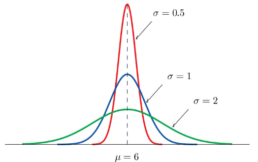
This figure illustrates how multiplying a random variable by a constant changes the spread of the distribution while leaving its center unchanged when no shift is applied. Source.
Effects on Variance
Since variance is the square of the standard deviation, the multiplicative effect on variability is stronger. Variance magnifies the effects of stretching or shrinking a distribution, and only a, not b, affects this measure.
EQUATION
= Variance of transformed variable
= Variance of original variable
= Scaling constant whose square determines variance change
Because variance intensifies differences, understanding this relationship is important when considering how transformations impact statistical modeling and probability assessments.
A connecting sentence: These changes to variance help students see how scale adjustments affect the overall dispersion of the transformed variable.
Interpreting Linear Transformations in Context
Interpreting the effects of linear transformations requires linking parameter changes to meaningful real-world scenarios. When the transformation rescales the variable, the units of measurement change, which can alter the interpretation of average outcomes and variability. Students should be attentive to these changes to maintain accurate contextual understanding.
Key points for interpretation include:
Additive shifts (b) move the entire distribution left or right without affecting variability.
Multiplicative scaling (a) changes the spread and potentially reverses direction.
Units of the transformed variable must be updated to match the transformation.
Shape remains constant, preserving the essential characteristics of the distribution.
These interpretive skills help students communicate statistical insights clearly and accurately across different contexts and transformed scales.
FAQ
A negative value of a produces a horizontal reflection of the distribution, meaning high values become low and vice versa.
This reflection can alter the interpretation of increasing or decreasing trends in the context of the variable.
For example, a negatively scaled test score would invert the ranking of performance.
However, the shape, spread (after accounting for the absolute value of a), and relative spacing of points remain unchanged.
Adding the same value to every observation shifts the entire distribution uniformly. All distances between data points remain identical.
As a result:
• The variance and standard deviation stay the same.
• The interquartile range, range, and other spread metrics are unaffected.
The only changes occur in location-based measures such as the mean, median, and quartiles.
Linear transformations cannot change skewness, modality, or tail behaviour. They preserve the overall structure of the distribution.
A skewed distribution remains skewed regardless of the constants a and b.
Similarly, peaks, gaps, or asymmetries remain present after transformation.
Transformations may adjust units or scales, but they do not correct distributional irregularities.
They allow data recorded in incompatible units to be expressed on a common scale without altering the statistical relationships within each dataset.
This ensures:
• Patterns within each variable remain intact.
• Measures such as correlation or relative rankings are preserved.
• Interpretations become clearer when variables originally measured in different units (for example, metres versus centimetres) need to be compared directly.
A linear transformation alters both the mean and standard deviation, so z-scores for the transformed variable no longer match those from the original variable.
However, once the transformed variable is standardised using its own mean and standard deviation, the resulting z-scores retain the same relative ordering as those from the original distribution.
The process of standardisation effectively removes the impact of a and b, returning the data to a scale with mean 0 and standard deviation 1.
Practice Questions
A random variable X has mean 12 and standard deviation 4. A new variable is created using the transformation Y = 3X + 5.
a) State the mean of Y.
b) State the standard deviation of Y.
a) Mean of Y = 3(12) + 5 = 41.
• 1 mark for correct substitution and calculation.
b) Standard deviation of Y = 3 × 4 = 12.
• 1 mark for applying scaling factor correctly.
A researcher records the weights (in kilograms) of parcels processed in a distribution centre, represented by the random variable X. The weights are then converted into grams using the transformation Y = 1000X.
a) Explain how this linear transformation affects the shape of the probability distribution.
b) Calculate the new mean and new standard deviation of Y, given that the mean of X is 2.5 kg and its standard deviation is 0.4 kg.
c) The researcher then adds a fixed packaging offset of 120 g to every value, forming Z = Y + 120. Describe the effect of this additional transformation on the mean and on the standard deviation.
a) The shape of the distribution remains unchanged; scaling by a constant stretches or compresses the distribution horizontally but does not alter its fundamental form.
• 1 mark for stating that the shape is preserved.
• 1 mark for describing stretch/compression due to scaling.
b) New mean of Y = 1000 × 2.5 = 2500 g.
New standard deviation of Y = 1000 × 0.4 = 400 g.
• 1 mark for correct mean.
• 1 mark for correct standard deviation.
c) Adding 120 increases the mean by 120 g but does not change the standard deviation.
• 1 mark for identifying change in mean only.
• 1 mark for stating standard deviation is unaffected.
