AP Syllabus focus:
‘UNC-3.B & UNC-3.B.1: Introduce the formula for calculating the probability of exactly x successes in n independent binomial trials with a success probability p, represented as P(X = x) = (n choose x) p^x (1 - p)^(n - x), where "n choose x" is the binomial coefficient. This subsubtopic focuses on understanding and applying the binomial probability formula to calculate specific probabilities within a binomial distribution context.’
This section develops the foundational skills needed to calculate probabilities in binomial settings, emphasizing how formulas model repeated, independent trials with constant success probability.
Calculating Binomial Probabilities
Understanding binomial probabilities is essential for studying random processes that involve repeated trials under consistent conditions. Because many real-world contexts involve scenarios with two outcomes and repeated attempts, the binomial model becomes a powerful tool for quantifying how likely specific results are.
Characteristics of a Binomial Setting
Before calculating binomial probabilities, it is crucial to ensure that the conditions defining a binomial random variable are present. A binomial random variable counts the number of successes in a fixed number of trials.

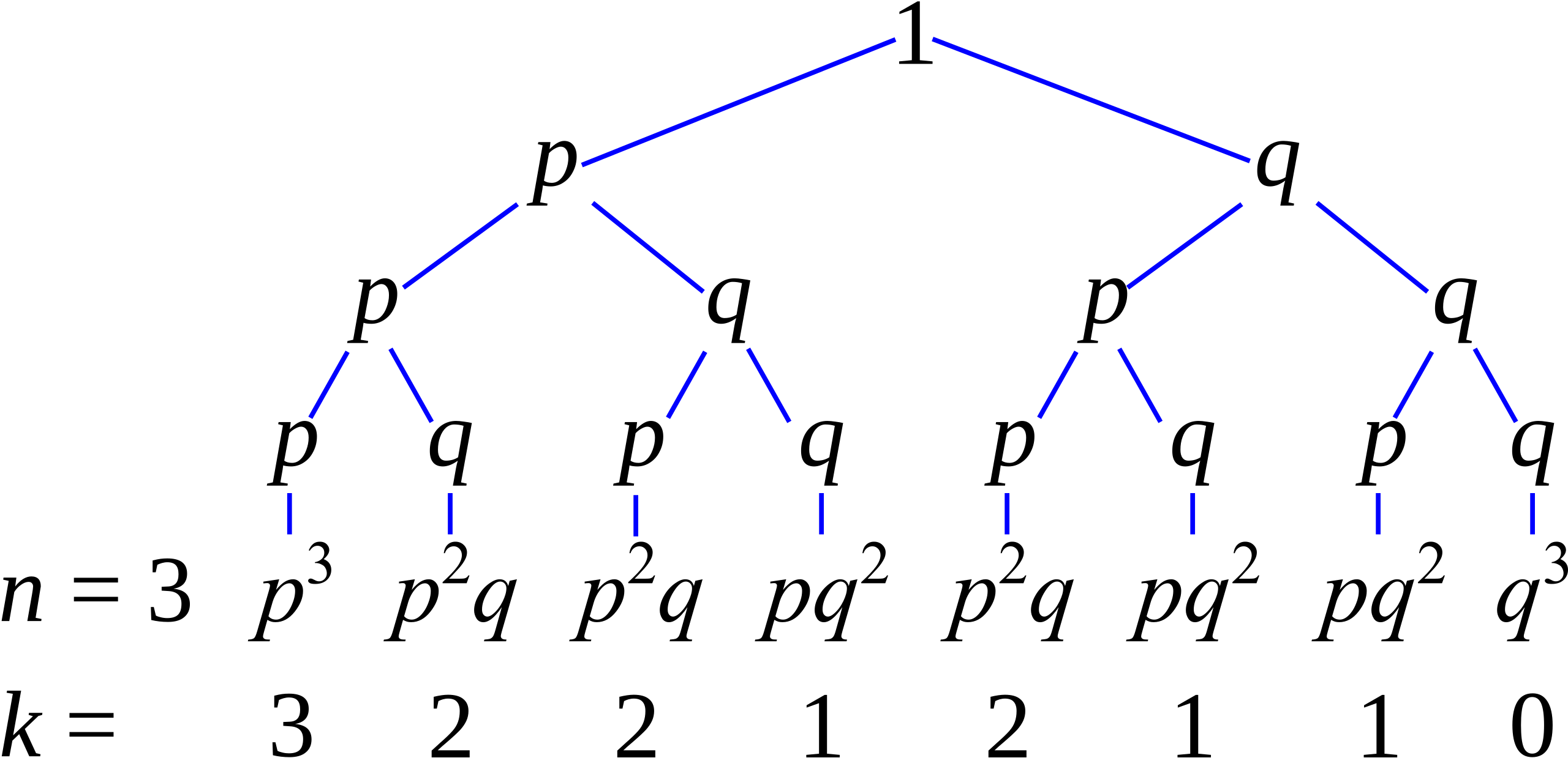
A probability tree illustrating independent repeated trials, each ending in success or failure with fixed probabilities, showing how sequences of outcomes form the basis of binomial modeling. Source.
Binomial Random Variable: A variable that counts the number of successes in n independent trials, each with two outcomes and constant success probability p.
A situation must satisfy the following conditions to be binomial:
A fixed number of trials is conducted.
Each trial results in one of two outcomes: success or failure.
The probability of success (p) remains constant across trials.
The trials are independent, meaning the outcome of one trial does not influence the outcome of another.
These criteria ensure that the binomial probability formula accurately models the behavior of the process.
The Binomial Probability Formula
Binomial probability calculations rely on a structured mathematical expression that accounts for the number of ways successes can occur and the probability of each arrangement.
EQUATION
= Probability of exactly successes
= Number of independent trials
= Number of successes of interest
= Probability of success on a single trial
= Probability of failure on a single trial
= Binomial coefficient counting the number of ways to arrange successes among trials
The formula includes two essential components:
The binomial coefficient, which counts how many possible sequences contain exactly x successes, and
The probability term, which multiplies the probabilities of successes and failures in a given sequence.
Together, these components capture both the structure and the likelihood of observing a specific number of successes.
Understanding the Binomial Coefficient
The binomial coefficient expresses how many distinct arrangements of successes and failures are possible when exactly x successes occur.

Pascal’s triangle displayed using binomial coefficient notation, showing how combinatorial values correspond to the number of possible success arrangements in a binomial setting. Source.
Binomial Coefficient: The number of distinct ways to choose x successes out of n trials, often read as “n choose x.”
Because each arrangement has the same probability under the binomial assumptions, the coefficient ensures that all valid configurations are counted when determining the total probability of exactly x successes.
A sentence such as the following helps reinforce the conceptual role of the binomial coefficient in probability calculations: it bridges the structure of repeated trials with the likelihood of observing specific patterns in those trials.
Interpreting Terms in a Binomial Probability
Each part of the binomial probability formula carries distinct meaning related to the behavior of repeated random processes:
The factor represents the contribution of all successes.
The factor represents the contribution of all failures.
The coefficient ensures all valid orders of successes and failures are counted.
These elements highlight how binomial probabilities synthesize both chance and combinatorics, creating a flexible tool for modeling repeated, independent events.

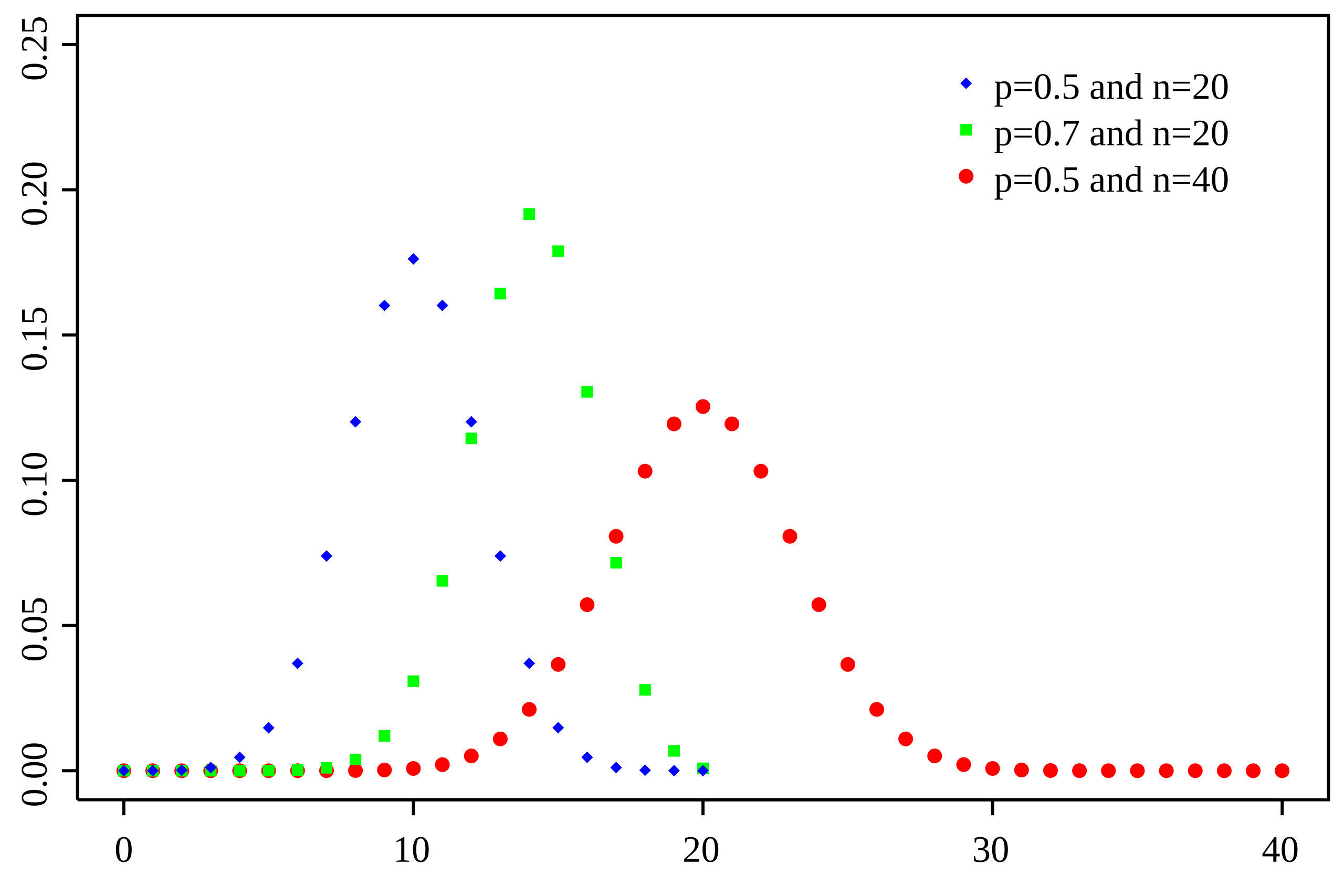
A probability mass function of a binomial distribution, showing discrete probability bars for each possible number of successes, illustrating how the binomial formula assigns a probability to every value of X. Source.
When to Apply the Binomial Probability Formula
Using the formula appropriately requires recognizing binomial structure in real contexts. To determine whether a situation qualifies:
Identify the success criterion clearly.
Confirm the number of trials is fixed.
Check that each trial has a consistent probability of success.
Ensure trials occur independently of each other.
If all conditions hold, the binomial probability formula provides an accurate and meaningful way to quantify the likelihood of observing exactly x successes.
Importance in Statistical Reasoning
Mastering binomial probability calculations strengthens understanding of how chance operates in repeated processes. Because many statistical methods rely on modeling random behavior using discrete probability distributions, the binomial framework forms a foundational building block for deeper study.
These notes emphasize that calculating binomial probabilities requires conceptual clarity about the structure of binomial trials and precise use of the associated formula, reinforcing the AP Statistics expectation of understanding and applying binomial reasoning.
FAQ
Look for language that suggests repeated attempts under identical conditions. Phrases such as “each attempt is independent”, “constant chance of success”, or “out of n trials” often indicate a binomial structure.
Also check whether the variable of interest is counting the number of successes rather than describing the sequence itself.
Each specific sequence of successes and failures has its own probability, and the binomial formula must account for all possible sequences that produce the same number of successes.
The probability of a single sequence might be straightforward to compute, but the total probability requires summing over every valid arrangement, which is why the binomial coefficient is essential.
The setting is no longer strictly binomial, because a binomial random variable requires a constant probability of success.
In practice, if the variation is minor and does not meaningfully affect expected outcomes, exam questions may still treat the scenario as approximately binomial. However, such approximations would always be stated or clearly implied in an AP context.
Independence ensures that one trial does not influence the outcome of another, allowing the binomial structure to work correctly.
Dependence arises when:
• Sampling is done without replacement from a small population.
• One individual’s outcome influences the next (such as learning effects or fatigue).
• External conditions change across trials.
It expresses the number of ways to select which x trials out of n are successes. This reflects a combinatorial idea: we care about which positions contain successes, not the specific nature of each failure.
Conceptually, it shows that probability in a binomial setting depends not only on chance but also on structure, because many arrangements may lead to the same observed count.
Practice Questions
Question 1 (1–3 marks)
A factory produces light bulbs, and each bulb has a 0.12 probability of being defective. A quality inspector tests 10 bulbs selected at random, assuming each test is independent.
Calculate the probability that exactly 2 of the 10 bulbs are defective.
Question 1 (1–3 marks)
• 1 mark: Identifies use of the binomial distribution (n = 10, p = 0.12, x = 2).
• 1 mark: Correctly substitutes into the binomial probability formula.
• 1 mark: Correct final probability value.
Question 2 (4–6 marks)
A basketball player takes 15 free throws. Each free throw is an independent trial with a probability of 0.7 of being successful. Let X be the number of successful free throws.
(a) Explain why X may be modelled as a binomial random variable.
(b) Calculate the probability that the player makes exactly 10 successful free throws.
(c) Calculate the probability that the player makes at least 12 successful free throws.
Question 2 (4–6 marks)
(a)
• 1 mark: States that each trial has two outcomes (success/failure).
• 1 mark: States that the number of trials is fixed and independent.
• 1 mark: States that the probability of success is constant.
(b)
• 1 mark: Correct identification of binomial model parameters (n = 15, p = 0.7, x = 10).
• 1 mark: Correct substitution into the binomial probability formula.
• 1 mark: Correct final probability value.
(c)
• 1 mark: Writes probability as P(X = 12) + P(X = 13) + P(X = 14) + P(X = 15).
• 1 mark: Correct substitution for all needed binomial probabilities.
• 1 mark: Correct final combined probability value.

