Parameters of a Geometric Distribution

A geometric distribution provides a powerful way to quantify how long it takes for the first success to occur in repeated independent trials. Understanding its mean and standard deviation helps describe the expected waiting time and how much that waiting time can vary.

Understanding What the Parameters Represent

The parameters of a geometric distribution summarize essential characteristics of how a random process behaves when repeated under the same conditions. Before exploring the formulas, it is important to clarify the role these parameters play in describing the variability of a geometric random variable.

The Role of Parameters in Describing a Distribution

The geometric distribution is based on a sequence of independent Bernoulli trials, each with a constant probability of success p. The random variable X counts how many trials are required until the first success occurs. Two parameters allow us to evaluate the central tendency and variability of this random behavior.

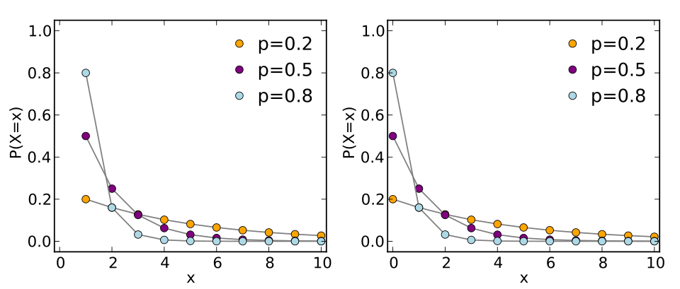
A set of geometric probability mass function plots showing how the distribution of waiting times changes with different success probabilities p. The points illustrate how larger p values generate higher probabilities for smaller trial counts, while smaller p values produce broader, more delayed distributions. Extra detail: the figure includes both common parameterizations of the geometric distribution, slightly beyond syllabus requirements but conceptually aligned. Source.

When the geometric distribution is introduced, students should understand that a parameter is a fixed numerical characteristic of a probability distribution that describes an entire population, not a single sample result. For the geometric setting, the most important parameters are the mean and the standard deviation, which describe the long-run behavior of repeated geometric experiments.

The Mean of a Geometric Distribution

The mean, or expected value, of a geometric random variable represents the average number of trials required to obtain the first success when the process is repeated many times. This value is not a prediction for any single trial sequence but a long-run average that captures the central tendency of the distribution.

EQUATION

This relationship highlights that as the probability of success increases, the expected waiting time decreases. Conversely, a small probability of success leads to a longer average wait for the first success.

Understanding this parameter is essential because it provides a baseline expectation for the process. Students should recognize that this expected value is a direct consequence of the independence and constant probability conditions that define geometric trials.

The Standard Deviation of a Geometric Distribution

While the mean captures the central value of the distribution, the standard deviation measures the typical distance between individual outcomes and the mean. For geometric distributions, this parameter describes how much the number of trials required for the first success tends to vary.

EQUATION

This formula shows that the standard deviation depends on both the chance of success and the structure of the geometric process. As p becomes larger, the denominator of the fraction grows more quickly, reducing the spread. When p is small, outcomes are more variable because long sequences of failures are more common, and the standard deviation correspondingly increases.

Interpreting Parameter Behavior

For AP Statistics students, it is important to interpret how changes in p affect both parameters:

• A larger p indicates more frequent successes.

  • The mean decreases, meaning fewer expected trials.

  • The standard deviation decreases, meaning outcomes vary less.

• A smaller p reflects rarer successes.

  • The mean increases, indicating longer expected waits.

  • The standard deviation increases, signaling greater variability.

These observations illustrate how geometric distribution parameters capture intuitive features of random processes with differing probabilities of success.

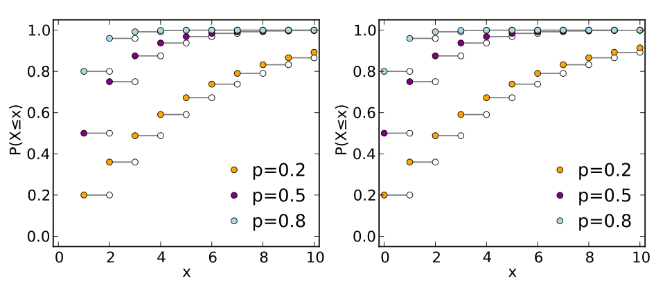
A set of geometric cumulative distribution function plots showing how quickly cumulative probability rises for different success probabilities p. Larger p values create steep early increases, reflecting shorter expected waiting times and lower variability. Extra detail: both common parameterizations of the geometric distribution are displayed, which slightly exceeds syllabus scope but supports conceptual understanding. Source.

Key Points for Application

The parameters of the geometric distribution provide essential information for interpreting real-world scenarios modeled with geometric behavior. To support correct academic understanding, students must be able to describe these ideas precisely.

Important points include:

• Both parameters depend entirely on p, emphasizing the role of the success probability.

• The mean describes typical waiting time; the standard deviation describes typical deviation from that waiting time.

• The interpretation of these parameters always uses units consistent with the context, such as “number of trials,” “number of attempts,” or any equivalent measure tied to the defined random variable.

• Parameters do not vary from one repetition of the process to another; they describe the theoretical distribution underlying all possible sequences of trials.

Why These Parameters Matter

These parameters are central in making sense of geometric distributions because they allow predictions about the long-run behavior of random processes involving waiting times. They guide statistical reasoning by characterizing both expected outcomes and the inherent uncertainty associated with chance processes. Understanding these parameters equips students to interpret and evaluate geometric models across a wide range of applied settings.