
AP Syllabus focus:
‘UNC-3.E.1: Explain the concept of a geometric random variable, X, as the count of trials until the first success in a sequence of independent Bernoulli trials, each with two possible outcomes: success or failure, and constant probability of success (p) and failure (1-p). This subsubtopic introduces the basics of geometric distribution and sets the stage for further exploration of its properties and applications.’
A geometric random variable captures how many repeated chance-based attempts occur before achieving a first success, emphasizing independence, constant probability, and the sequential nature of Bernoulli trials.
Defining Geometric Random Variables
A geometric random variable arises from a specific type of random process governed by Bernoulli trials, in which each trial has only two possible outcomes. Because students frequently encounter repeated chance situations, such as continued attempts until an event occurs, understanding this structure is essential for later probability and distribution topics.
Term: A geometric random variable is a random variable that counts the number of trials needed to obtain the first success in repeated, independent Bernoulli trials with constant probability of success.
This understanding builds directly on the AP Statistics expectation that students recognize how repeated, identical conditions create predictable long-run probabilistic structures. Within this framework, geometric random variables provide a model for “waiting time” scenarios, where the value of the random variable represents not an outcome from a single trial but the position of the first success in a sequence.
Structure of Bernoulli Trials
A geometric random variable is only valid when generated from Bernoulli trials, which are experiments characterized by repeated attempts with consistent conditions. For a process to be modeled using the geometric distribution, it must satisfy several necessary constraints rooted in the syllabus requirement.
Characteristics of Bernoulli Trials
Each trial in the sequence must meet all of the following conditions:
Two outcomes only: Each trial results in either success or failure, with no additional categories allowed.
Constant success probability: The probability of success, denoted p, remains unchanged from trial to trial.
Constant failure probability: The probability of failure remains 1 – p, complementing the fixed success probability.
Independence: The outcome of one trial must not influence the outcome of the next.
Sequential counting of trials: Trials continue until the first success occurs.
Term: Bernoulli trial: A single random experiment with only two outcomes—success or failure—performed under identical, independent conditions.
These structural criteria ensure that the geometric random variable aligns with the AP specification’s emphasis on independence and consistent probabilities. Because dependence or changing probabilities disrupts the geometric pattern, students must be careful to identify whether the scenario truly meets all assumptions.
A geometric random variable arises from a sequence of independent Bernoulli trials, where each trial has two possible outcomes (success or failure) and the probability of success stays the same from trial to trial.
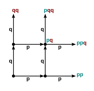
Tree diagram illustrating successive Bernoulli trials with branches labeled for success (p) and failure (q), showing how sequences of failures and eventual success are formed. Path labels provide additional detail beyond this subsubtopic by previewing later probability calculations for geometric distributions. Source.
Understanding the “Count of Trials” Perspective
A defining feature of geometric random variables is how they count. Instead of measuring how many successes occur within a fixed number of attempts, they measure when the first success occurs. This makes geometric random variables fundamentally different from binomial random variables, which require a fixed number of trials. The geometric setting continues potentially without limit, making the support of the random variable the set of positive integers.
Ordering and Interpretation
The position of the first success is meaningful because:
Each additional trial represents another independent opportunity.
The probability structure shifts based on how many failures precede the first success.
The value of the geometric random variable reflects a waiting time, measured in discrete increments.
This perspective reinforces the importance of independent repetition and steady probability. Without these, the count of trials until first success cannot be described with the geometric framework.
Probability Foundations of Geometric Random Variables
Although this section does not compute geometric probabilities explicitly, the AP syllabus expects students to understand the conceptual basis. Because each trial has a constant probability of success, the probability that the first success occurs on a specific trial depends on repeated failure followed by one eventual success. This characteristic shape—rooted in repeated (1 – p) failures—illustrates why geometric distributions are closely connected to exponential decay patterns in probability.
EQUATION
= A positive integer counting trial occurrence, measured in discrete units
A single sentence ensures a smooth transition before introducing additional structural ideas.
Because each trial is identical and independent, the possible values of X are the positive integers 1, 2, 3, …, and the chance that the first success occurs on a later trial gets smaller and smaller.
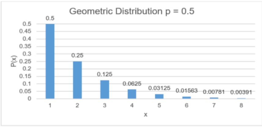
Bar graph depicting a geometric distribution with p = 0.5, where the highest probability occurs at X = 1 and declines as X increases. Numerical labels above each bar offer probability values that extend slightly beyond this definitional subsubtopic while remaining consistent with the behavior of geometric random variables. Source.
Conditions Required for Geometric Modeling
When determining whether a scenario can be modeled using a geometric random variable, students should evaluate whether all necessary criteria are satisfied. A process is geometric only when:
The interest is in the first success, not multiple successes.
Trials are performed under identical conditions.
The likelihood of success is the same on every trial.
Each trial is independent of previous results.
The sequence theoretically continues indefinitely until success occurs.
Understanding these conditions establishes a strong foundation for later sections involving probability calculations, mean and standard deviation of geometric distributions, and interpretations within real-world contexts.
FAQ
A situation fails to be geometric if any core condition is violated.
Common violations include:
• The probability of success changes after each attempt (learning, fatigue, or adaptive difficulty).
• The trials are not independent (success makes future attempts more likely).
• There is more than one type of success or failure outcome.
If any of these occur, the waiting time for a first success will not follow a geometric pattern.
The value represents the number of trials required to achieve a first success.
It is impossible to obtain a success before conducting any trials, so zero cannot be a valid outcome.
Some textbook contexts define alternative versions that start at 0, but the AP specification uses the standard definition where the minimum value is 1.
Geometric random variables are memoryless, meaning the probability of success on the next trial is unaffected by previous failures.
This matters because it ensures that the waiting time has the same probabilistic structure no matter how many failures have occurred.
Only the geometric and exponential distributions have this property in common.
Geometric models fit situations where you repeatedly try something until it works.
Typical examples include:
• Reattempting a password until correct.
• Calling a phone number until someone answers.
• Shooting basketball free throws until the first score.
Each scenario must satisfy independence and constant probability, not just repeated attempts.
It helps estimate expected waiting times for first-time events under stable conditions.
This is particularly helpful when deciding whether to modify processes:
• If the waiting time is long, it may indicate low success probability and encourage redesign.
• If it is short and predictable, the process may be operating efficiently.
Practice Questions
Question 1 (1–3 marks)
A factory runs independent quality checks on its products. Each check has a constant probability of 0.12 of detecting a defect.
(a) Explain why the number of checks required until the first defect is detected can be modelled using a geometric random variable.
(2 marks)
Question 1
(a) (2 marks total)
• 1 mark: States that each trial (quality check) has only two outcomes: defect detected or not detected.
• 1 mark: States that trials are independent and have a constant probability of success (detecting a defect), so the number of trials until the first success fits a geometric model.
Question 2 (4–6 marks)
A basketball player takes repeated free throws during practice. Each shot is independent, and the probability she scores on any given attempt is 0.7.
(a) State the conditions required for the number of attempts until her first successful shot to follow a geometric distribution.
(2 marks)
(b) Explain why the number of attempts until her first successful shot is a geometric random variable.
(2 marks)
(c) State the possible values that this geometric random variable can take and briefly describe what large values of the variable represent.
(2 marks)
Question 2
(a) (2 marks total)
• 1 mark: Identifies that each attempt must have only two outcomes (success or failure).
• 1 mark: Identifies that attempts are independent and the probability of success must remain constant across trials.
(b) (2 marks total)
• 1 mark: States that the situation involves repeated, identical, independent attempts.
• 1 mark: States that the variable counts the number of attempts until the first success, matching the definition of a geometric random variable.
(c) (2 marks total)
• 1 mark: States that the possible values are the positive integers: 1, 2, 3, and so on.
• 1 mark: Correctly explains that large values correspond to many consecutive failures occurring before the first successful shot.
