
AP Syllabus focus:
‘The interval estimate for the difference between two sample proportions (p̂1 - p̂2) is found using the formula: (p̂1 - p̂2) ± z* √((p̂1(1-p̂1)/n1) + (p̂2(1-p̂2)/n2)), where p̂1 and p̂2 are the sample proportions, n1 and n2 are the sample sizes, and z* is the z-score corresponding to the desired confidence level.’
Calculating the Confidence Interval
A confidence interval for the difference between two population proportions provides a statistically supported range of plausible values. It quantifies sampling variability and supports comparisons.
Understanding the Purpose of a Two-Proportion Confidence Interval
A two-sample confidence interval estimates the difference between two population proportions, expressed as p̂1 − p̂2, allowing researchers to determine how two groups compare based on sample evidence. This interval is centered on a point estimate, which is the numerical difference between the sample proportions, and expands outward using a margin of error that reflects uncertainty due to sampling.
Components Required for the Interval
Constructing a confidence interval demands accurate identification of several essential elements that are grounded in sample data and the desired confidence level. These elements ensure the computation captures realistic variability in categorical responses.
The Point Estimate
The point estimate for the difference in population proportions is the observed difference in the two sample proportions. This value serves as the foundation of the interval and represents the best single estimate before incorporating uncertainty.
Point Estimate (Difference of Proportions): The observed difference between two sample proportions, calculated as p̂1 − p̂2.
This point estimate summarizes the observed comparative behavior of the groups based solely on the sample.
The Standard Error of the Difference
The standard error quantifies expected variability in the difference between sample proportions from sample to sample. It incorporates information about the spread within each group and adjusts for sample sizes.
EQUATION
= Sample proportions for groups 1 and 2
= Sample sizes for groups 1 and 2
Understanding this standard error supports recognition of how sample sizes and sample proportions directly affect the width of the final interval.
Identifying the Critical Value
The critical value, denoted z*, reflects the selected confidence level and determines how far from the point estimate the interval extends.
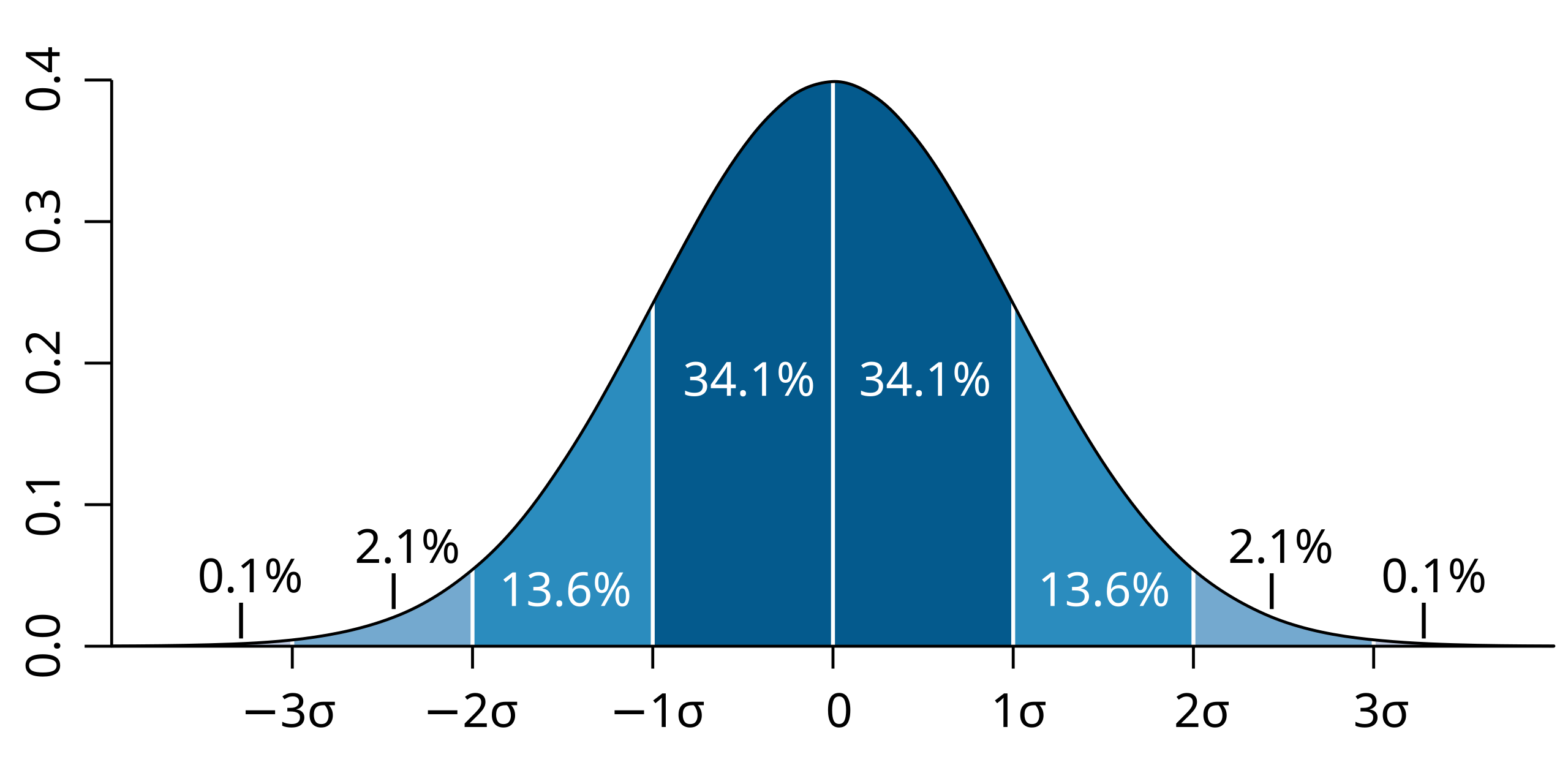
This diagram illustrates the standard normal distribution with marked standard deviation intervals, showing how proportions of data fall within ±1, ±2, and ±3 standard deviations—concepts that relate directly to selecting z* for a confidence level. Source.
Larger critical values correspond to higher confidence levels because more certainty demands a wider range of plausible differences. Students should recognize that z* arises from the standard normal distribution, which models standardized sampling distributions under appropriate conditions.
Constructing the Margin of Error
The margin of error incorporates both sampling variability and desired certainty. It depends on the standard error and the critical value, forming a key component of the full interval.
EQUATION
= Margin of error (scale of sampling uncertainty)
= Critical value tied to chosen confidence level
A well-defined margin of error signals how much the estimate may reasonably differ from the actual population difference.
Assembling the Confidence Interval
The confidence interval integrates the point estimate and margin of error to form a symmetric range of plausible differences between population proportions. This structure highlights the statistical reasoning that the true difference is unlikely to lie far from the observed sample difference.
EQUATION
= Point estimate for difference in proportions
This interval expresses the balance between sample evidence and uncertainty, offering a clear window into how groups may differ at the population level.
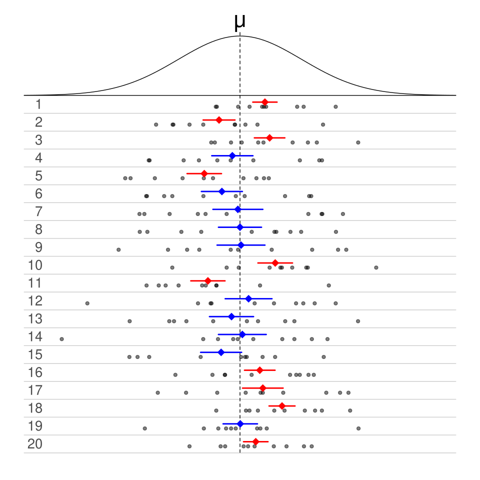
Each horizontal bar represents a confidence interval for repeated samples, visually demonstrating that some intervals will contain the true parameter while others will not—capturing the long-run interpretation of confidence intervals. Source.
Interpretation in Context
The computed interval must be interpreted in the study’s context. An interval entirely above zero suggests that the first population proportion is likely higher, whereas an interval entirely below zero suggests the opposite. An interval containing zero indicates that no difference is supported by the sample data within the confidence level chosen. A contextually grounded interpretation ensures that statistical reasoning aligns meaningfully with real-world questions.
Factors Influencing Interval Width
Several factors affect the width of a two-proportion confidence interval, each linked to the components of the standard error and margin of error.
Sample Size
Larger sample sizes reduce the standard error term, thereby narrowing the interval. This reduction occurs because proportion estimates become more stable with more observations.
Sample Proportions
Proportions near 0.5 typically produce greater variability, widening the interval. Proportions near 0 or 1 often reduce variability, slightly narrowing the interval.
Confidence Level
Higher confidence levels require larger z* values, expanding the interval to ensure greater certainty.
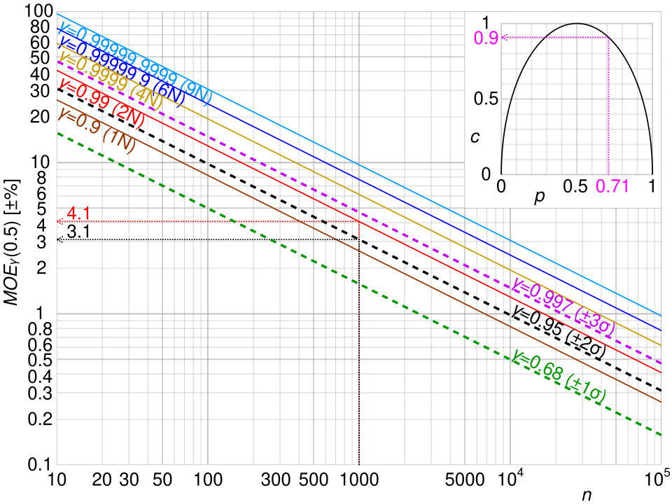
The graph displays how margin of error decreases as sample size increases and increases with higher confidence levels, reinforcing the relationships that shape interval width for two-proportion confidence intervals. Source.
These factors interact to shape the final interval and determine how precisely the difference between two population proportions can be estimated.
FAQ
Because p̂1 − p̂2 is a direct, unbiased estimate of the true difference between the two population proportions, it aligns neatly with the idea of comparing categories across groups.
Using this simple difference ensures the interpretation remains clear: positive values indicate one group has a higher proportion, while negative values indicate the opposite.
Unequal sample sizes influence each group’s contribution to the standard error.
Larger samples reduce variability more effectively, so a group with a much larger n will have a stronger stabilising effect on the interval.
Smaller samples introduce more uncertainty, often causing the interval to widen.
The variability of a proportion is greatest when the proportion is close to 0.5 and smaller when it is near 0 or 1.
This affects the standard error because the product p̂(1 − p̂) shrinks as the sample proportion moves toward the extremes.
As a result, intervals may become narrower when sample proportions lie near the boundaries of the scale.
Large differences in p̂1 and p̂2 do not invalidate the method, but they can increase variability in the estimate.
The more important considerations are:
• Adequate sample sizes in both groups
• Independence within and between groups
• Meeting the normality condition for both samples
If these conditions hold, the interval remains appropriate.
Independence ensures the variability from one group does not influence the other, allowing the standard error formula to combine their variances correctly.
If samples are not independent, the estimated standard error may be too small or too large, causing misleadingly narrow or wide intervals.
This results in confidence intervals that do not achieve the stated confidence level and may yield incorrect inferences.
Practice Questions
Question 1 (1–3 marks)
A researcher compares the proportion of customers who prefer Brand A in two independent shops. In Shop 1, 48 out of 120 customers prefer Brand A. In Shop 2, 30 out of 90 customers prefer Brand A.
(a) Identify the point estimate for the difference in population proportions (p1 − p2).
(b) State the formula for the standard error of the difference between two sample proportions used when constructing a confidence interval.
Question 1
(a) 1 mark
• Correct calculation of the point estimate: (48/120) − (30/90) = 0.40 − 0.33 = 0.07
Award 1 mark for identifying 0.07 or an equivalent expression.
(b) 1–2 marks
• 1 mark for stating the general form of the standard error:
SE = sqrt( p1(1 − p1)/n1 + p2(1 − p2)/n2 )
• Award full 2 marks if the response clearly states that this formula is used when constructing a confidence interval for the difference between two population proportions.
Total: 2–3 marks
Question 2 (4–6 marks)
A public health analyst wants to estimate the difference in the proportion of adults who meet daily exercise recommendations in two neighbouring cities. A random sample of 400 adults from City X shows that 62% meet the recommendations, while a random sample of 350 adults from City Y shows that 55% meet them.
(a) Calculate the margin of error for a 95% confidence interval for the difference in population proportions, using the appropriate components.
(b) Construct the 95% confidence interval for pX − pY.
(c) Interpret the interval in context, explaining what it suggests about the difference in exercise habits between the two cities.
Question 2
(a) 1–2 marks
• 1 mark for correctly identifying the components of the margin of error:
Use z* = 1.96 for a 95% confidence level,
SE = sqrt( pX(1 − pX)/nX + pY(1 − pY)/nY ).
• 1 mark for correctly substituting values into the structure of the margin of error formula:
ME = 1.96 × SE.
Do not award marks for numerical calculation.
(b) 2 marks
• 1 mark for stating the confidence interval structure:
(pX − pY) ± ME.
• 1 mark for substituting the sample proportions 0.62 and 0.55 into the interval expression.
No numerical computation required.
(c) 1–2 marks
• 1 mark for correctly interpreting the interval in context, referring to the difference between the two cities’ proportions.
• 1 mark for noting whether the interval suggests a meaningful difference (e.g., that City X appears to have a higher proportion meeting the recommendations if the interval lies above zero, or that evidence of a difference is uncertain if the interval includes zero).
Total: 4–6 marks
