
AP Syllabus focus:
‘Conditions include: a) Linearity between x and y, checked by residual analysis. b) Constant standard deviation of y for all x, also checked by residuals. c) Independence of data, ensured by random sampling or experiments, and the 10% condition for sampling without replacement. d) Normality of y-values for any x, with n > 30 if data is skewed.’
Confidence intervals for a regression slope are only valid when specific statistical conditions hold. Verifying these conditions ensures that inferences about the population slope are trustworthy and meaningful.
Verifying Conditions for Confidence Intervals for the Slope
Constructing a confidence interval for the population slope requires confirming that the data meet conditions ensuring the accuracy of regression-based inference. These conditions focus on the behavior of the relationship between variables, the distribution of errors, and the structure of the data. When these requirements are satisfied, the resulting interval reliably reflects uncertainty in estimating the true slope.
Linearity Condition
The linearity condition requires that the relationship between the explanatory variable x and the response variable y is genuinely linear. This ensures that the regression model y = a + bx appropriately represents the form of the relationship.
Students verify linearity using residual analysis, which evaluates whether deviations from the fitted line follow a random scatter rather than a systematic curve.
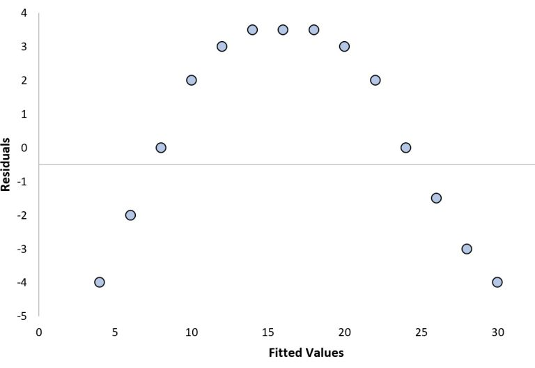
Residual plot showing a curved pattern, indicating violation of the linearity condition because the residuals do not scatter randomly around zero. Source.
Residuals: The differences between observed values and predicted values, calculated as . Residuals measure deviations from the fitted regression line.
A properly satisfied linearity condition is indicated by a residual plot showing no curvature or pattern. Any clear structure in the residuals signals that a linear model does not adequately describe the data.
Constant Standard Deviation (Homoscedasticity)
For regression inference, the standard deviation of y must remain constant across all values of x. This property, known as homoscedasticity, is also evaluated using a residual plot. Students look for a uniform vertical spread of residuals, avoiding patterns such as funnels or fans, which suggest heteroscedasticity.
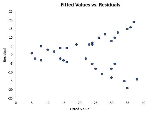
Residual plot with a funnel-shaped spread of points, demonstrating heteroscedasticity where error variability increases with fitted values, violating the constant standard deviation condition. Source.
Homoscedasticity: The condition in which the variability of residuals is approximately the same for all values of the explanatory variable.
When the spread of residuals changes with x, the standard error of the slope may be inaccurate, undermining the validity of the confidence interval.
Independence of Observations
The independence condition ensures that each data point provides unique information. This requirement is typically met by collecting data through random sampling or random assignment in experiments. Independence is essential because regression formulas assume that errors are not systematically related to one another.
A key guideline used in AP Statistics is the 10% condition, which applies when sampling without replacement.
10% Condition: When sampling without replacement, the sample size must be less than 10% of the population to maintain approximate independence.
Proper study design remains the most reliable way to ensure independence; residual analysis cannot diagnose dependence effectively.
Normality of y-Values for Each x
To construct a t-based confidence interval for the slope, the distribution of y-values at each fixed x should be approximately normal. While perfect normality is unnecessary, large departures—especially strong skewness or outliers—can distort estimates of the slope’s variability.
When sample sizes are sufficiently large, the Central Limit Theorem helps mitigate moderate non-normality. The syllabus emphasizes a practical guideline: if the data are skewed, a sample size greater than 30 supports the normality condition for inference.
EQUATION
= Standard deviation of the residuals
= Individual x-values
= Mean of x-values
This standard error measures the variability of slope estimates across repeated samples and depends on the assumption that the distribution of errors is approximately normal.
A well-behaved normal probability plot of residuals provides support for meeting the normality condition. Severe deviations such as long tails or sharp peaks suggest caution in interpreting the resulting confidence interval.
Integrating the Conditions in Practice
These four conditions—linearity, constant standard deviation, independence, and normality—collectively establish whether a t-interval for the slope is justified. Residual plots serve as the primary diagnostic tool for the first two conditions, whereas study design ensures independence and distributional checks support normality. When all conditions are reasonably met, the resulting confidence interval accurately reflects uncertainty in estimating the population slope.
FAQ
Look for consistent direction changes. Random scatter should show points distributed without forming bends, waves, or repeating shapes. Even slight curvature across the x-axis indicates a potential violation of linearity.
Check whether residuals systematically shift from positive to negative across x-values. Subtle non-linearity often appears as a gentle arc rather than a dramatic curve.
Smoothing lines (such as lowess curves) can help reveal hidden structure, though they are not required for the AP exam.
When sampling without replacement, residuals can become correlated if the sample makes up too large a proportion of the population. The 10% condition minimises this dependency.
In regression, correlated residuals undermine the validity of standard error estimates for the slope, which rely on independence. Ensuring the sample is less than 10% of the population helps preserve approximate independence.
Mild skewness is generally acceptable, especially with moderate or large samples, because slope estimates remain stable. Strong skewness becomes problematic when it introduces influential points or distorts the distribution of residuals.
A practical sign of problematic skewness is when extreme residuals appear on a normal probability plot or when a few points heavily affect the fitted line.
Residual plots isolate model errors rather than showing the overall relationship. Patterns in residuals are easier to detect because the linear trend has already been removed.
Scatterplots may hide non-linearity or heteroscedasticity when the relationship is strong. Residuals magnify departures from assumptions, making them more reliable for diagnosing conditions required for inference.
Yes. Outliers can distort the slope and artificially reduce patterns in residuals, giving the impression of acceptable conditions.
Effects include:
• Inflated or deflated standard error of the slope
• Masked curvature or hidden heteroscedasticity
• Distortion of the normality assessment
When an outlier influences the fitted line, condition checks should be reconsidered with and without the point.
Practice Questions
Question 1 (1–3 marks)
A student constructs a residual plot after fitting a least-squares regression line. The plot shows a curved pattern with residuals systematically above the line for low x-values and below the line for mid-range x-values.
(a) Identify which condition for constructing a confidence interval for the slope is violated.
(b) Explain why this violation makes a confidence interval for the slope inappropriate.
Question 1
(a) 1 mark
• Identifies the linearity condition as the one violated.
(b) 1–2 marks
• States that the curved pattern indicates the relationship is not linear (1 mark).
• Explains that this makes inference inappropriate because the regression model does not accurately describe the underlying relationship, making slope estimates unreliable (1 mark).
Total: 2–3 marks
Question 2 (4–6 marks)
A researcher collects a random sample of 45 observations to study the relationship between daily temperature and electricity usage. After fitting a linear regression model, they examine the following information:
• The residual plot shows a roughly constant vertical spread across all x-values.
• The sample was selected using simple random sampling from a population of thousands.
• A normal probability plot of the residuals shows slight skew but no major outliers.
• The residual plot shows no curved pattern.
(a) For each of the four conditions required for constructing a confidence interval for the slope, state whether the condition is met and justify your answer.
(b) Explain whether it would be appropriate to construct a confidence interval for the slope in this situation.
Question 2
(a) Up to 4 marks
• Linearity: States it is met because there is no curved pattern in the residual plot (1 mark).
• Constant standard deviation: States it is met because the vertical spread in the residual plot is roughly constant (1 mark).
• Independence: States it is met because simple random sampling was used and the population is large, satisfying the 10% condition (1 mark).
• Normality: States it is reasonably met because the sample size is large (45) and the normal probability plot shows only slight skew and no major outliers (1 mark).
(b) Up to 2 marks
• States that constructing a confidence interval for the slope is appropriate because all conditions are reasonably satisfied (1 mark).
• Provides justification that the model assumptions for using the t-based interval hold in practice (1 mark).
Total: 4–6 marks
