
AP Syllabus focus:
‘The point estimate for the slope is b, the observed slope from data. The confidence interval for the slope is given by b ± (t* × SE), where t* is the critical value from the t distribution for the desired confidence level and SE is the standard error of the slope.’
Confidence intervals for regression slopes quantify uncertainty in estimating the population slope, helping students understand how sample-based results generalize to the broader population under appropriate conditions.
Calculating Confidence Intervals for the Slope
A confidence interval for a regression slope provides a range of plausible values for the population slope (β) based on the sample slope (b).
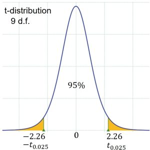
This t-distribution diagram highlights the central confidence region and tail probabilities, illustrating how a chosen confidence level determines the critical value t∗t^*t∗ used in constructing the interval b±t∗×SEb \pm t^* \times SEb±t∗×SE. Although originally shown in the context of means, the same distributional concept applies directly to slope estimation in regression. Source.
This subsubtopic focuses on the procedure for constructing that interval and the ideas that justify it, emphasizing the role of sampling variability and the use of the t-distribution when estimating a regression coefficient.
The Point Estimate: The Sample Slope
The point estimate is the single best estimate of the population slope and is always the observed slope from the sample regression line, denoted by b.
Point Estimate (Slope): The statistic b, calculated from sample data, used to estimate the population slope β in a simple linear regression model.
Because any sample represents only one of many possible random samples, b varies from sample to sample. This variability is captured by the standard error of the slope, which plays a central role in constructing a confidence interval.
Understanding the Standard Error of the Slope
The standard error of the slope (SE) measures the typical deviation of sample slope estimates from the true population slope when repeated samples are taken using the same method.
Standard Error of the Slope: A statistic measuring the variability of the sample slope b as an estimator of the population slope β.
A smaller standard error indicates more precise estimation, which produces narrower confidence intervals. The standard error depends on the spread of the data around the regression line and the variability of the explanatory variable.
Structure of a Confidence Interval for the Slope
A confidence interval incorporates both the point estimate and the uncertainty around it. Because the true population slope is unknown and the standard error is estimated from data, the interval uses the t-distribution rather than the normal distribution.
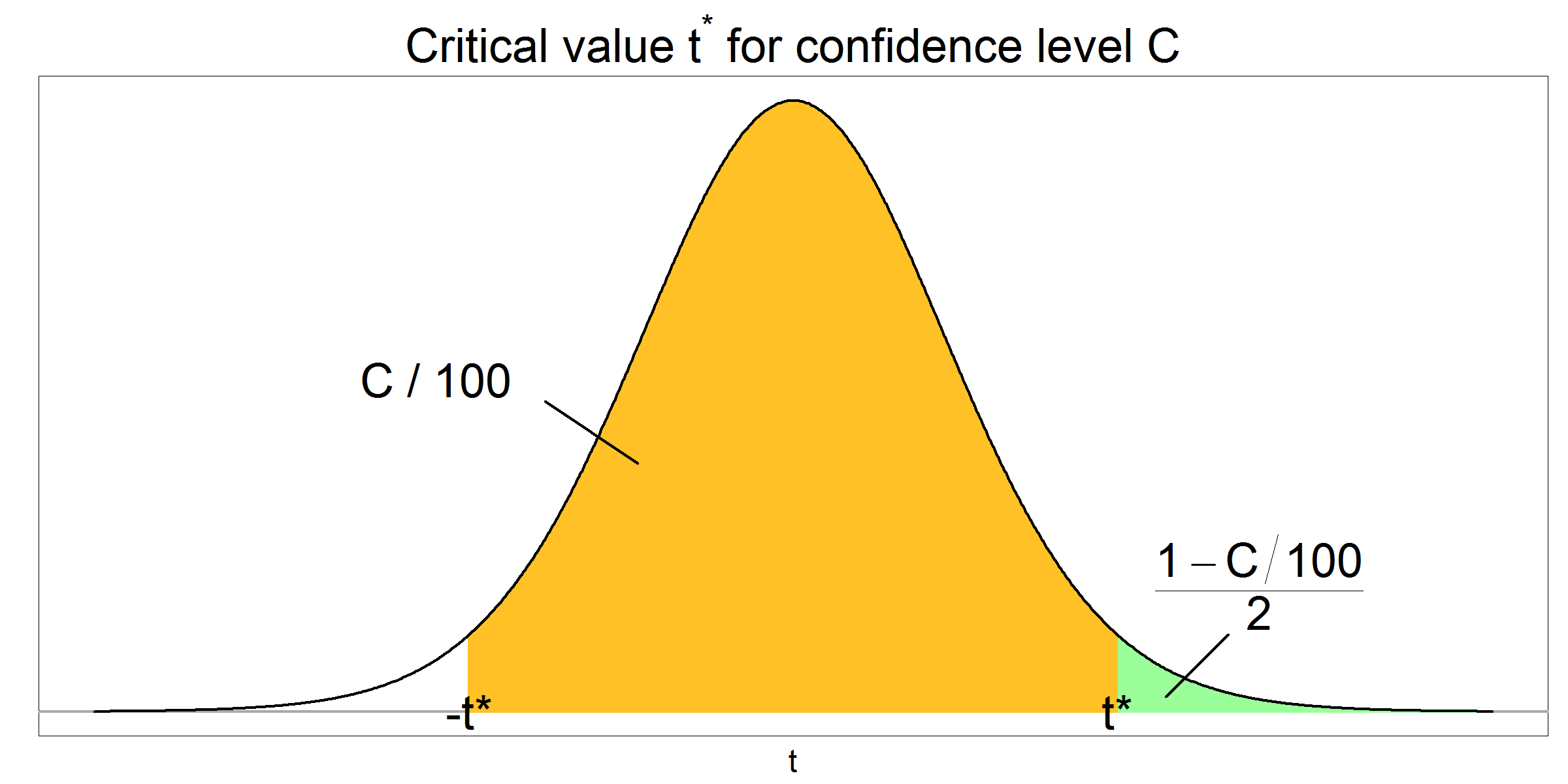
This diagram shows how the central confidence level and symmetric tail regions define the critical values ±t*. It reinforces that selecting a confidence level determines the cutoff values used in the interval formula for the slope. Although general, it directly parallels the procedure for regression slope confidence intervals. Source.
EQUATION
= Sample slope, the point estimate for the population slope
= Critical value from the t-distribution for the chosen confidence level
= Standard error of the slope, representing variability in slope estimates
This form aligns with the general structure of confidence intervals: estimate ± margin of error. The t-distribution accounts for additional uncertainty when the population standard deviation is unknown, which is always the case in real regression settings.
A confidence interval communicates uncertainty in a probabilistic sense: under repeated sampling, approximately C% of intervals constructed using this method will contain the true population slope β, if all statistical conditions are satisfied.
Components Needed to Construct the Interval
Students should recognize the three essential components required:
Point estimate (b)
Represents the observed slope for the sample.Critical value (t*)
Depends on the confidence level and degrees of freedom (n − 2 for simple linear regression). Higher confidence levels correspond to larger critical values and therefore wider intervals.Standard error (SE)
Quantifies variability in slope estimates across samples.
These components combine to form a defensible numerical range for the population slope.
Interpreting the Critical Value t*
The critical value reflects how confident we want to be that the true slope lies within the calculated interval.
A higher confidence level requires capturing more of the distribution, which increases the value of t∗t^*t∗. This results in wider confidence intervals, reflecting greater caution in capturing the true population slope.
Margin of Error for the Slope
The margin of error measures the extent of uncertainty around the point estimate. Larger margins reflect more uncertainty.
Margin of Error (Slope): The product of the critical value t* and the standard error SE, representing the maximum expected difference between the sample slope b and the true slope β under repeated sampling.
The margin of error widens when the sample size is small, the confidence level is high, or the data show substantial scatter around the regression line.
Why the t-Distribution Is Used
In regression, the variability of the slope estimate depends on the variability of the residuals and the distribution of the explanatory variable. Because the population standard deviation of residuals is unknown, we rely on the sample-based estimate. This introduces uncertainty that the t-distribution appropriately models, particularly when sample sizes are modest.
Steps for Constructing the Confidence Interval
Students should follow a structured approach when building a confidence interval for the slope:
Identify the sample slope (b) from the regression output.
Locate the standard error of the slope (SE).
Determine the degrees of freedom (n − 2).
Choose the desired confidence level.
Obtain the critical value t* from the t-distribution.
Compute the interval using b ± (t* × SE).
Each step reflects a direct application of the specification’s emphasis on the relationship between the estimate, the standard error, and the critical value drawn from the t-distribution.
Importance of the Confidence Interval
A confidence interval for the slope supports meaningful statements about the direction and strength of a linear relationship in the population. By grounding interpretation in the sample and acknowledging the uncertainty inherent in estimation, the interval becomes a powerful inferential tool aligned with the goals of AP Statistics.
FAQ
A higher confidence level widens the interval because it requires capturing a larger proportion of plausible slope values. This means the estimate becomes less precise but more reliable in covering the true population slope.
In contrast, a lower confidence level narrows the interval, offering greater precision but increasing the risk that the interval does not include the true slope.
Sample size affects the standard error of the slope. Larger samples reduce random variation in slope estimates, producing smaller standard errors and narrower intervals.
Smaller samples inflate the standard error, leading to wider intervals that reflect greater uncertainty about the population slope.
Values close to zero suggest weak evidence for a linear relationship between the variables, even if the interval includes both positive and negative slopes.
Interpretation should consider:
• Whether zero is inside the interval
• How close endpoint values are to zero
• Whether the relationship is practically meaningful in the given context
Outliers can distort both the slope estimate and the standard error, potentially pulling the interval away from the true population value or inflating its width.
If an outlier strongly influences the regression line, the resulting confidence interval may misrepresent the underlying linear relationship and exaggerate uncertainty.
A sample slope alone gives only a single estimate, offering no indication of precision or uncertainty.
A confidence interval:
• Shows how much the slope might vary across samples
• Indicates whether the direction of the relationship is clearly supported
• Helps judge the practical significance of the estimated effect
Practice Questions
Question 1 (1–3 marks)
A researcher fits a least-squares regression line to data relating hours of study (x) and exam score (y). The sample slope is 2.4, and the standard error of the slope is 0.8.
Construct a 95% confidence interval for the slope using a critical value of t* = 2.12.
Interpret the interval in context.
Question 1 (1–3 marks)
• 1 mark: Correct use of the confidence interval formula b ± t* × SE.
• 1 mark: Correct numerical interval: 2.4 ± (2.12 × 0.8) = 2.4 ± 1.696, giving (0.704, 4.096). Allow minor rounding errors.
• 1 mark: Contextual interpretation stating that the researcher is 95% confident that the true population slope lies within this interval, meaning each additional hour of study is associated with an increase in exam score between roughly 0.7 and 4.1 points.
Total: 3 marks.
Question 2 (4–6 marks)
A company investigates the relationship between temperature (x, in degrees Celsius) and the strength of a chemical solution (y). A regression analysis produces the following output:
• Sample slope b = −0.37
• Standard error of the slope SE = 0.11
• Sample size n = 28
(a) Calculate a 99% confidence interval for the slope using a critical value of t* = 2.77.
(b) Explain what this interval suggests about the relationship between temperature and solution strength.
(c) Comment on whether the interval provides evidence that increasing temperature reduces average solution strength in the population.
Question 2 (4–6 marks)
(a)
• 1 mark: Correct set-up of confidence interval: b ± t* × SE.
• 1 mark: Correct margin of error calculation: 2.77 × 0.11 = 0.3047 (or equivalent rounding).
• 1 mark: Correct interval: −0.37 ± 0.305 → (−0.675, −0.065). Allow minor rounding differences.
(b)
• 1 mark: Interpretation stating that the interval suggests the true population slope is negative, indicating that higher temperatures are associated with lower average solution strength.
• 1 mark: Interpretation must explicitly refer to the population and acknowledge uncertainty (e.g., “We are 99% confident…”).
(c)
• 1 mark: Clear statement that the entire interval is below zero, providing evidence that increasing temperature reduces mean solution strength in the population.
• 1 mark: Justification referencing the negativity of all plausible slope values in the interval.
Total: 6 marks.
