This subsubtopic develops the essential skill of computing a regression slope test statistic, enabling inference about population relationships using sample-based estimates and modeled variation.

Understanding the Purpose of the Test Statistic

The test statistic for a regression slope quantifies how far the sample slope deviates from a hypothesized population slope, relative to the slope’s estimated variability.

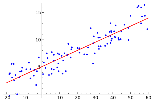
Scatterplot of data points with a fitted linear regression line. The line represents the estimated relationship between the explanatory and response variables, with its slope serving as the point estimate bbb used in the test statistic. This image focuses on the fitted line and random variation around it without adding procedures beyond those required in the syllabus. Source.

This measure allows students to compare observed results against what would be expected if the null hypothesis were true, anchoring slope-based inference in the t-distribution, which appropriately models sampling variation when estimating parameters from sample data.

Before calculating the test statistic, it is important to clarify what the slope represents. In simple linear regression, the population slope β represents the average change in the response variable for each one-unit increase in the explanatory variable. When a research question involves testing a claim about this relationship, the slope becomes the focal point for significance testing.

The calculation of the test statistic depends on the comparison between the observed slope and the hypothesized value under the null hypothesis. Students should recall that the sample slope b serves as an unbiased estimate of β, and that its variability is expressed through the standard error of the slope, denoted SE_b.

Components Required for the Test Statistic

Three essential elements are needed to compute the test statistic:

• Sample slope (b): Obtained from regression output and used as the point estimate.

• Hypothesized slope (β₀): The value specified by the null hypothesis, often 0 when testing for no linear association.

• Standard error of the slope (SE_b): Measures variation in slope estimates across repeated samples.

These components work together to standardize the difference between b and β₀, expressing it in units of estimated standard deviation. This standardization allows comparison to the t-distribution.

Students must ensure that conditions for regression inference are satisfied. While this subsubtopic does not require verifying conditions in detail, the validity of the resulting t-statistic depends on assumptions such as linearity, independence, constant variability of residuals, and approximate normality of the response distribution for each x-value.

Calculating the Test Statistic Using the t-Distribution

The slope test statistic follows the t-distribution with n − 2 degrees of freedom, reflecting the two parameters (intercept and slope) estimated during regression. The t-distribution is appropriate because the population standard deviation of residuals is unknown and must be estimated from the sample.

EQUATION

This formula computes how many standard errors separate the observed slope from the hypothesized value. A larger absolute t-value indicates stronger evidence against the null hypothesis, as the observed slope appears farther from the hypothesized slope than would typically occur by chance.

After computing the t-statistic, it is interpreted using the t-distribution with n − 2 degrees of freedom, which governs how sample-to-sample variation behaves when estimating a regression slope.

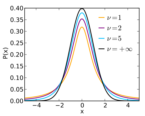
Plot of probability density functions for several Student’s t-distributions with different degrees of freedom. The curves are bell-shaped and centered at zero, emphasizing that the t-statistic for the slope is compared to this family of distributions when making inferences. The image also shows multiple degrees of freedom simultaneously, which goes slightly beyond the syllabus requirement but helps visualize how the t-distribution changes as sample size increases. Source.

This distribution captures uncertainty arising from finite sample sizes and is more spread out than the normal distribution, particularly for smaller n.

Interpreting the Meaning of the Test Statistic

Although this subsubtopic focuses on calculation rather than interpretation, understanding its role within inference strengthens comprehension. The magnitude of the t-statistic reflects how unusual the observed slope would be if the null hypothesis were true. The direction (positive or negative) indicates whether the sample slope is above or below the hypothesized slope.

A complete significance test requires comparing this statistic to critical values or determining a p-value, but those steps belong to later subsubtopics. Here, students must master the computation itself and the reasoning that the statistic quantifies deviation relative to estimated variability.

Process for Computing the Test Statistic

Students can follow a structured process:

• Identify the observed slope b from regression output.

• Determine the hypothesized slope β₀ from the null hypothesis.

• Obtain the standard error SE_b from the regression analysis.

• Compute the t-statistic using the formula $(b - \beta_0)/SE_b$.

• Recognize that the resulting statistic follows a t-distribution with n − 2 degrees of freedom.

Each step contributes to forming a standardized measure that reflects how plausible the observed slope is under the assumption that the null hypothesis is correct.