
AQA Specification focus:
‘The Keynesian AS curve.’
Introduction
The Keynesian Aggregate Supply (AS) curve illustrates how national output responds to changes in aggregate demand across different phases of economic activity, especially under varying levels of spare capacity.
The Keynesian Aggregate Supply Curve: An Overview
The Keynesian AS curve is distinct from the classical vertical long-run AS curve. It reflects Keynesian perspectives on how economies function in the short run, particularly during recessions or periods of underemployment. Unlike the classical view that assumes markets clear quickly, Keynesian analysis accepts that wages and prices may be sticky, meaning the economy can remain below full employment for extended periods.
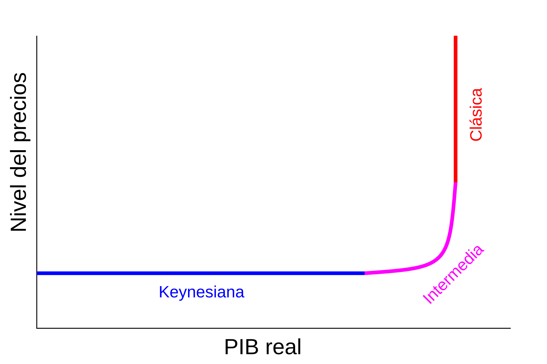
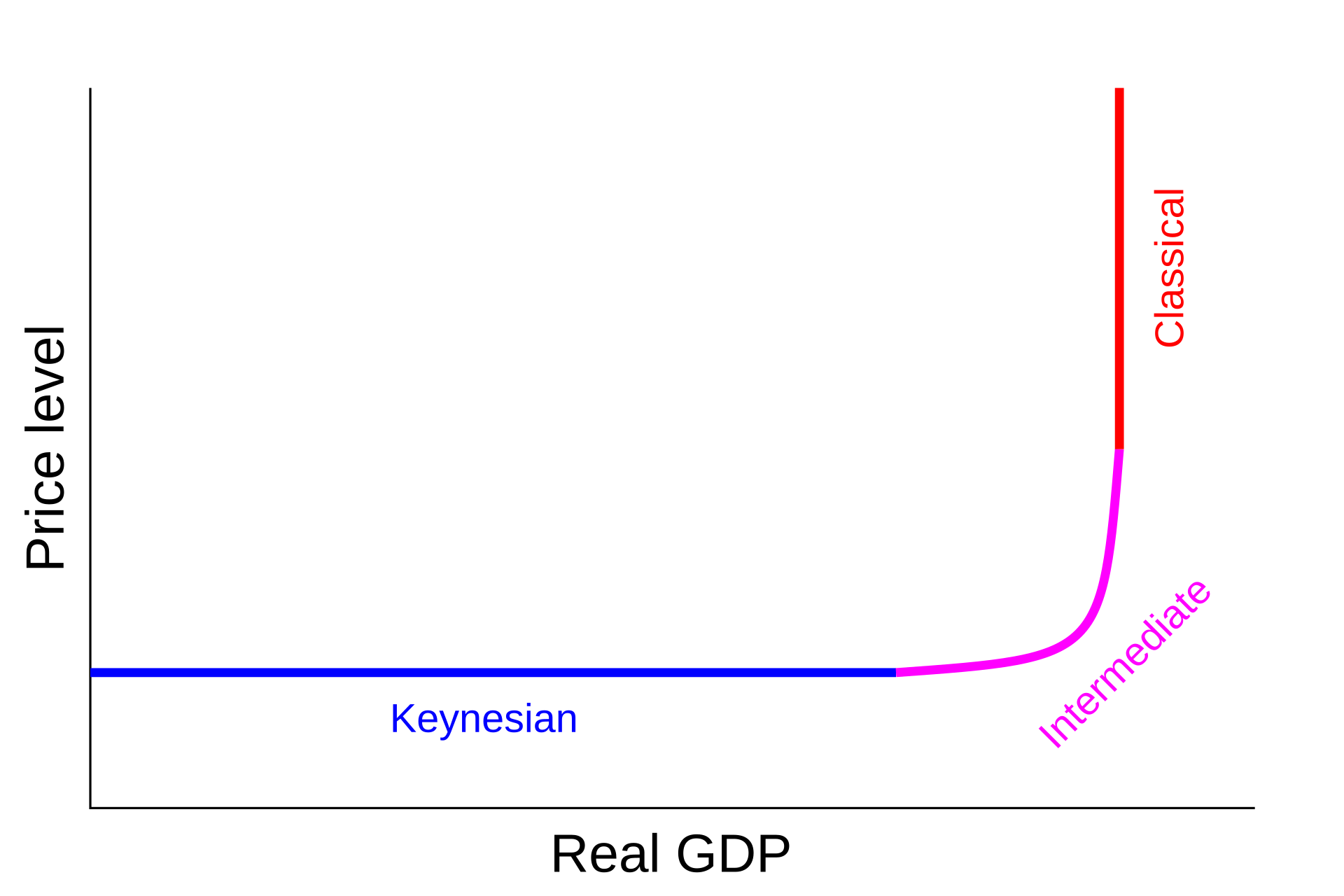
The Keynesian AS curve is therefore non-linear, with three main sections that represent different economic conditions:
Horizontal (Keynesian range) at low levels of output.
Upward-sloping (intermediate range) as spare capacity is gradually used up.
Vertical (full capacity range) when the economy reaches maximum productive capacity.
This diagram depicts the Keynesian Aggregate Supply curve, highlighting the horizontal, upward-sloping, and vertical sections that correspond to varying levels of economic output and inflationary pressures. It demonstrates how the economy can function below full capacity with limited inflation, supporting Keynesian economic theory. Source
Structure of the Keynesian AS Curve
1. Horizontal Section (Low Output and High Unemployment)
In this section, the curve is flat.
Spare capacity is extensive, meaning resources such as labour and capital are underutilised.
Increases in aggregate demand (AD) can lead to higher output without upward pressure on the price level.
This reflects Keynes’s belief that economies can operate below full employment for long periods.
Spare capacity: The underutilisation of resources, where labour and capital are not employed to their full potential.
2. Intermediate Section (Rising Output with Inflationary Pressure)
Here, the AS curve slopes upwards.
As AD increases, output rises, but some bottlenecks appear in certain industries.
Rising costs of production (e.g., overtime pay, higher raw material demand) begin to exert inflationary pressure.
This stage illustrates the transition towards full employment.
3. Vertical Section (Full Employment Output)
The AS curve becomes vertical, indicating the economy is at full productive capacity.
Any further increase in AD will lead only to inflation rather than growth in real output.
This aligns with the classical view of the economy in the long run.
Full employment: The level of output where all available resources (labour, capital, land, and entrepreneurship) are fully utilised without generating excessive inflation.
Why the Keynesian Curve Matters
The Role of Sticky Wages and Prices
Keynes argued that wages and prices are sticky downwards due to contracts, minimum wage laws, and resistance from workers and firms. This means the economy may not automatically adjust to restore equilibrium. As a result, governments may need to intervene to stimulate demand when output is below potential.
Government Intervention
The Keynesian model justifies demand-side policies such as fiscal stimulus, since increases in AD can expand output without raising inflation when the economy is in the horizontal section of the AS curve.
Examples of interventions:
Fiscal policy: Increased government spending or tax cuts.
Monetary policy: Lowering interest rates to boost consumption and investment.
Supply-Side Constraints
As output rises towards full employment, supply-side constraints become more binding. Productivity, labour market flexibility, and investment in capital all influence where the economy sits on the Keynesian AS curve.
The Keynesian AS Curve and Economic Performance
Illustrating Different States of the Economy
Recession: The economy operates in the horizontal range, meaning large increases in AD can boost output without inflation.
Recovery: As growth accelerates, the economy moves into the upward-sloping section, where inflationary pressures build.
Boom: At full capacity, the economy hits the vertical range, where growth is constrained, and inflation rises with further demand.
Demand-Side vs Supply-Side Influences
The Keynesian AS curve helps economists distinguish between issues caused by insufficient demand and those caused by structural supply-side limitations.
Demand deficiency keeps the economy in the flat range.
Supply shortages shift the curve leftward, reducing capacity and causing inflation at lower levels of output.
This illustration shows the aggregate supply curve encompassing the Keynesian, intermediate, and classical ranges, offering a broader context for understanding how the economy transitions between different phases of output and inflation. It aids in distinguishing between demand deficiencies and supply-side constraints. Source
Shifts in the Keynesian AS Curve
Factors that Shift the Curve Outwards (Right)
Technological progress improving productivity.
Increased investment in capital stock.
Education and training raising labour quality.
Improved efficiency in resource allocation.
Factors that Shift the Curve Inwards (Left)
Rising production costs such as higher oil prices.
Supply shocks (e.g., natural disasters, wars).
Institutional weaknesses like inefficient financial systems that restrict business funding.
Supply-side shock: An unexpected event that suddenly changes the cost of production or availability of resources, shifting the aggregate supply curve.
Linking the Keynesian Curve to Policy and Debate
Keynesian vs Classical Views
Keynesians argue that active intervention is necessary to lift economies from recessions and avoid prolonged underemployment.
Classical economists believe the economy self-corrects in the long run through flexible markets, making intervention unnecessary.
Modern Policy Relevance
The Keynesian AS curve remains central to debates over fiscal policy, especially in times of crisis such as financial recessions or pandemics. It highlights how increases in demand can stimulate growth without inflation when spare capacity is high.
Practice Questions
Identify two characteristics of the horizontal section of the Keynesian Aggregate Supply (AS) curve. (2 marks)
Award 1 mark for each valid characteristic (maximum 2 marks).
Possible answers:
Represents a period of high unemployment/spare capacity (1 mark).
Output can increase without upward pressure on the price level (1 mark).
Resources are underutilised (1 mark).
Prices are sticky or do not rise despite increases in aggregate demand (1 mark).
Explain how an increase in aggregate demand affects output and the price level as the economy moves along the three sections of the Keynesian Aggregate Supply (AS) curve. (6 marks)
Level 1 (1–2 marks): Basic statements with little or no development. For example: “Output rises when demand increases.”
Level 2 (3–4 marks): Some development with reference to two sections of the curve, but limited depth. For example: “In the flat section, output increases without inflation. In the vertical section, only prices rise.”
Level 3 (5–6 marks): Clear, well-structured explanation covering all three sections of the curve. For example:
Horizontal section: Output rises significantly with no inflation due to spare capacity (1–2 marks).
Intermediate section: Both output and prices rise as resources are increasingly utilised (1–2 marks).
Vertical section: Only prices rise since the economy is at full capacity (1–2 marks).
FAQ
The Keynesian AS curve reflects situations of unemployment and spare capacity, which classical theory overlooks. It acknowledges that wages and prices may be sticky and not adjust quickly.
This makes it better at explaining long periods of low growth without inflation, such as recessions, where economies operate far below potential output.
Periods of severe recession or depression, such as the Great Depression of the 1930s or the 2008–09 global financial crisis, illustrate this section.
Output and employment were far below potential.
Stimulus policies increased demand without generating inflation.
Supply-side improvements shift the curve rightward, allowing the economy to produce more without immediate inflation.
Examples include:
Investment in new technology.
Improvements in worker skills and training.
Infrastructure development.
These raise the economy’s capacity, expanding the flat and intermediate ranges before inflationary pressure builds.
As resources become scarcer, firms must pay higher wages, compete for inputs, or use less efficient resources.
This pushes up costs, meaning both output and prices rise together. Inflation emerges gradually before full employment is reached.
Policymakers use it to justify intervention during downturns. When the economy is in the flat section, fiscal or monetary expansion can raise output with minimal inflation.
In contrast, if the economy is already near the vertical section, similar policies risk fuelling inflation rather than boosting real growth.
