Geometric Distribution is an essential concept in probability theory and is particularly useful in the study of discrete random variables. It deals with the probability of encountering the first success in a sequence of independent Bernoulli trials, each with the same probability of success.

Definition and Characteristics

Geometric Distribution is characterized by its focus on the number of trials needed to achieve the first success. It's defined by a single parameter, $p$, which is the probability of success in each trial. Key features include:

• The trials are independent of each other.
• The probability of success, $p$, remains constant in every trial.
• It counts the trials until the first success.

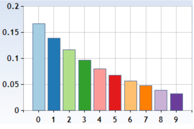
Image courtesy of brilliant.org

Theoretical Foundation

This distribution is grounded in the concept of Bernoulli trials, where each trial has two possible outcomes: success or failure. Geometric Distribution is a model for scenarios where these trials are repeated until success is achieved for the first time.

Geometric Probability Formula

The probability mass function (PMF) for a geometrically distributed variable $X$ is:

Here, $x$ is the number of trials, and $p$ is the probability of success on each trial.

Example Problems

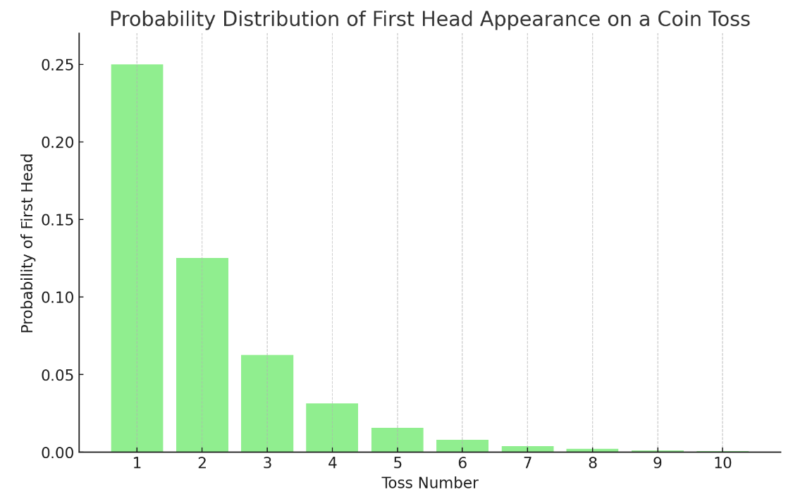
Example 1: Coin Toss Scenario

Consider a fair coin (probability of heads = 0.5) tossed repeatedly until heads is obtained. Find the probability that the first head appears on the 3rd toss.

Solution:

Using the geometric probability formula:

1. Calculate $(1 - p)^{x - 1}$, which is $(1 - 0.5)^{3 - 1} = 0.5^2 = 0.25$.

2. Multiply this by $p$, which is 0.5 in this case. So, $0.25 \times 0.5 = 0.125$.

Therefore, the probability of the first head appearing on the third toss is 12.5%.

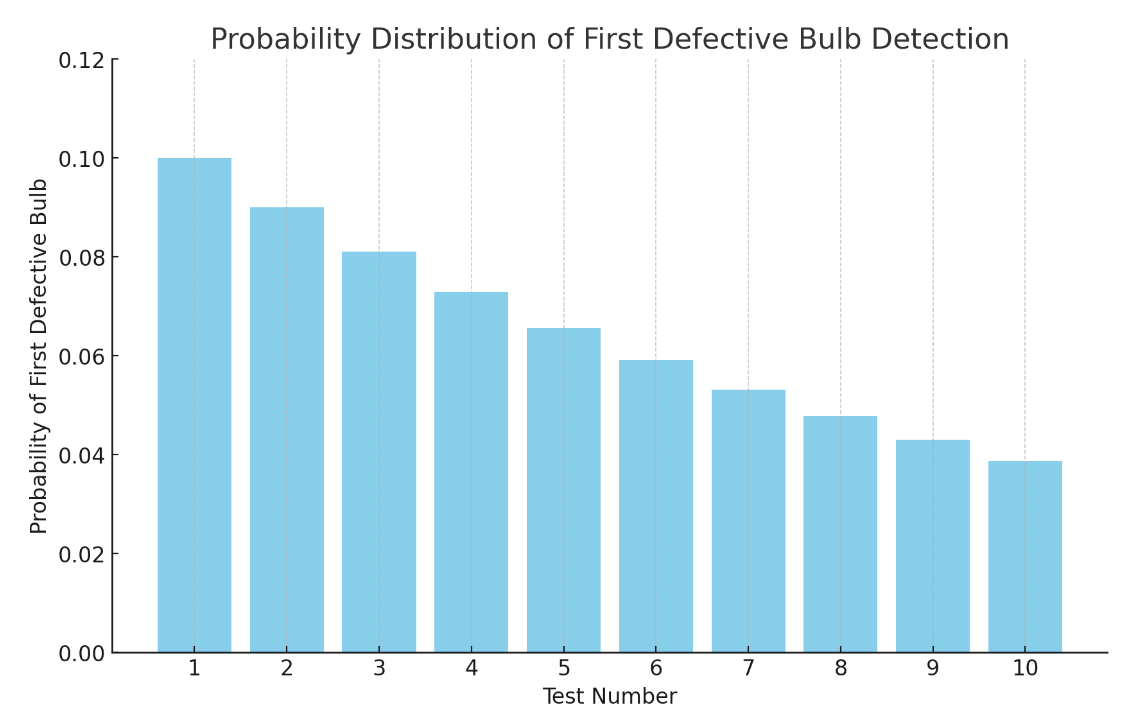
Example 2: Quality Control in Manufacturing

In a factory, the probability of a bulb being defective is 0.1. Find the probability that the first defective bulb is detected on the 5th test.

Solution:

Applying the formula:

1. Compute $(1 - p)^{x - 1}$, which is $(1 - 0.1)^{5 - 1} = 0.9^4$. This equals approximately 0.6561.

2. Multiply this by $p$, which is 0.1. So, $0.6561 \times 0.1 \approx 0.06561$.

Hence, there's a 6.56% chance that the first defective bulb will be found on the 5th bulb tested.