
OCR Specification focus:
‘Use the Hardy–Weinberg principle to calculate allele, genotype and phenotype frequencies in populations under stated assumptions.’
The Hardy–Weinberg principle provides a mathematical framework to study how allele and genotype frequencies behave in populations. It assumes equilibrium conditions where evolutionary forces do not act.
The Hardy–Weinberg Principle
The Hardy–Weinberg principle describes the genetic structure of a population that is not evolving. It predicts that allele and genotype frequencies will remain constant from one generation to the next, provided that specific conditions are met. This principle forms a fundamental baseline for understanding population genetics and evolutionary change.
Hardy–Weinberg Equilibrium: The state of a population in which allele and genotype frequencies remain stable across generations, in the absence of evolutionary influences.
When a population is in Hardy–Weinberg equilibrium, any changes in allele frequencies over time indicate that one or more assumptions have been violated, such as natural selection or genetic drift acting on the population.
Assumptions of the Hardy–Weinberg Model
The equilibrium model is based on several key assumptions. These assumptions define an idealised population in which allele frequencies remain constant.
Large population size – to prevent random fluctuations in allele frequencies (minimising genetic drift).
No mutations – no new alleles arise through DNA changes.
No migration – no gene flow in or out of the population.
Random mating – individuals mate independently of genotype.
No selection – all alleles confer equal reproductive success.
In reality, these conditions are rarely all met simultaneously. However, deviations from the equilibrium provide important evidence for evolutionary processes in natural populations.
Allele and Genotype Frequencies
In a population, each gene locus may have two or more forms of a gene, known as alleles. For a locus with two alleles, represented by A and a, the Hardy–Weinberg principle can predict the proportion of different genotypes.
Allele Frequency: The relative proportion of a particular allele among all alleles of that gene in a population.
EQUATION
—-----------------------------------------------------------------
Hardy–Weinberg Equation (Alleles) = p + q = 1
p = frequency of dominant allele (no units)
q = frequency of recessive allele (no units)
—-----------------------------------------------------------------
This equation expresses the idea that the sum of all allele frequencies for a gene equals one. From this, we can derive the frequencies of possible genotypes.
EQUATION
—-----------------------------------------------------------------
Hardy–Weinberg Equation (Genotypes) = p² + 2pq + q² = 1
p² = frequency of homozygous dominant genotype (AA)
2pq = frequency of heterozygous genotype (Aa)
q² = frequency of homozygous recessive genotype (aa)
—-----------------------------------------------------------------
These relationships enable biologists to predict the distribution of genotypes within a population if allele frequencies are known, or vice versa.
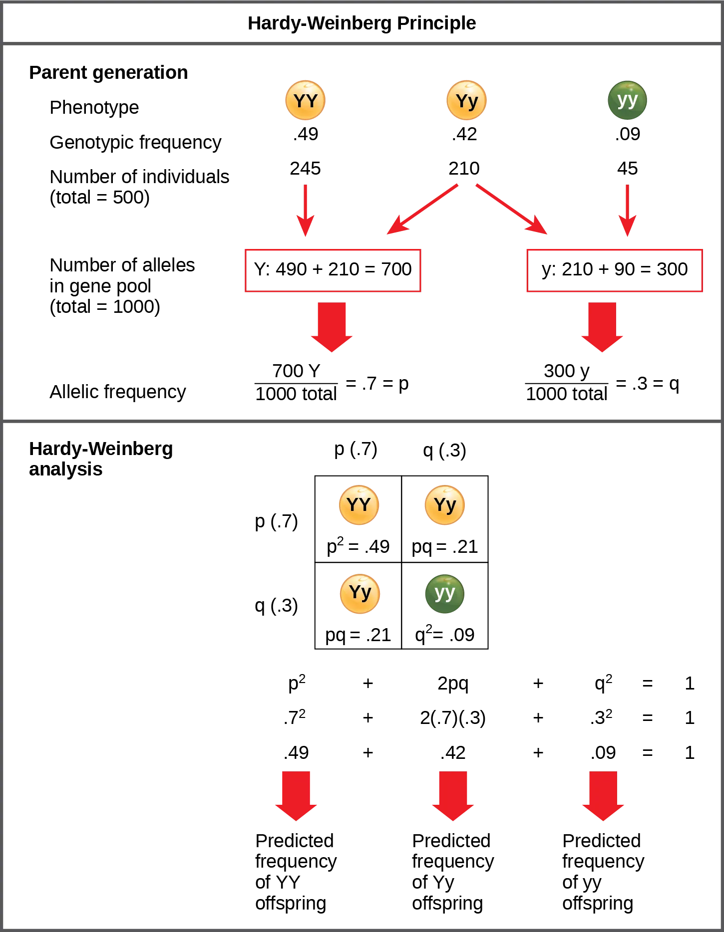
Figure 19.2 illustrates how allele frequencies (p and q) determine expected genotype frequencies (p², 2pq, q²) under Hardy–Weinberg equilibrium. The diagram reinforces that, when assumptions are met, genotype proportions predicted from allele frequencies remain stable across generations. If field data deviate from these expected values, evolutionary forces are implicated. Source.
Predicting Population Genetic Structure
The Hardy–Weinberg equations are useful for calculating:
Allele frequencies from observed genotype data.
Expected genotype frequencies when allele frequencies are known.
Phenotype frequencies if dominance relationships are known.
For example:
If q² represents individuals showing a recessive phenotype, the square root of q² gives q, and then p = 1 – q.
These values can be substituted into p² + 2pq + q² = 1 to calculate all genotype proportions.
This Punnett square shows how random mating in a large population yields the genotype frequencies p² (AA), 2pq (Aa), and q² (aa). It visualises the binomial expansion underlying Hardy–Weinberg equilibrium and clarifies why genotype proportions follow from allele frequencies. The layout is intentionally minimal to emphasise calculation. Source.
Such calculations allow scientists to assess whether observed data match expected equilibrium values.
Applications of the Hardy–Weinberg Principle
The principle is a foundational tool in population genetics. It allows researchers to:
Detect whether evolutionary change is occurring.
Identify selective pressures or genetic drift effects.
Estimate the frequency of carriers for recessive genetic diseases.
Monitor changes in allele frequencies in conservation biology.
In human genetics, it helps estimate the proportion of heterozygous carriers for inherited conditions such as cystic fibrosis or sickle-cell anaemia. In ecology, it aids in assessing genetic diversity within wild populations.
Factors That Disrupt Hardy–Weinberg Equilibrium
When real populations deviate from the idealised model, it indicates that one or more assumptions are violated. Common factors disrupting equilibrium include:
Mutation
Introduction of new alleles through DNA sequence changes.
Alters existing allele frequencies gradually over generations.
Gene Flow
Movement of individuals between populations.
Introduces or removes alleles, changing frequency patterns.
Genetic Drift
Random fluctuations in small populations.
May lead to allele fixation or loss purely by chance.
Non-Random Mating
Includes inbreeding, assortative mating, or sexual selection.
Changes genotype frequencies without necessarily altering allele frequencies.
Natural Selection
Differential reproductive success alters allele frequencies.
Favours alleles that confer survival or reproductive advantages.
Using the Hardy–Weinberg Model to Detect Evolutionary Change
When comparing observed genotype frequencies with those predicted by Hardy–Weinberg equilibrium, any significant deviation suggests that evolution may be occurring. For example:
A shift in allele frequencies might indicate selection.
An excess of homozygotes could indicate inbreeding.
A loss of genetic variation may suggest genetic drift in small populations.
Thus, the model provides a null hypothesis for population genetics — assuming no evolution, any deviations indicate the influence of evolutionary forces.
Limitations of the Hardy–Weinberg Principle
Although the principle is powerful, it is an idealised mathematical model. Its assumptions are rarely met fully in natural populations. Some key limitations include:
It does not account for multiple alleles or polygenic traits.
It assumes diploid organisms with sexual reproduction.
It overlooks effects of mutation rates, migration intensity, and selection strength that may vary in time and space.
Nevertheless, despite its simplifications, the Hardy–Weinberg principle remains a cornerstone for understanding genetic stability and change within populations, underpinning much of modern evolutionary biology.
Practice Questions
Question 1 (2 marks)
State two assumptions of the Hardy–Weinberg principle that must be met for a population to remain in genetic equilibrium.
Mark Scheme
1 mark for each correct assumption (maximum 2 marks).
Accept any two of the following:
• The population is large (no genetic drift).
• No mutations occur.
• No migration or gene flow occurs.
• Random mating takes place.
• No selection occurs (all genotypes equally likely to survive and reproduce).
Question 2 (5 marks)
In a population of beetles, the allele for green colour (G) is dominant over the allele for brown colour (g).
The population is in Hardy–Weinberg equilibrium.
If 9% of the beetles are brown, calculate the frequency of the dominant allele (G).
Explain the steps in your calculation and describe what the Hardy–Weinberg principle tells us about this population.
Mark Scheme
Award marks as follows:
1 mark – Recognises that 9% brown beetles means q² = 0.09.
1 mark – Calculates q = 0.3 (square root of 0.09).
1 mark – Calculates p = 1 – q = 0.7 (frequency of dominant allele).
1 mark – Explains that Hardy–Weinberg assumes allele and genotype frequencies remain constant over generations in the absence of evolutionary influences.
1 mark – States that the population is in equilibrium, meaning no selection, mutation, migration, or genetic drift is acting on the allele frequencies.
FAQ
Scientists compare observed genotype frequencies from a population with the expected frequencies calculated using the Hardy–Weinberg equation.
If the observed and expected frequencies differ significantly, this suggests that at least one equilibrium condition has been violated.
Possible causes include:
Natural selection favouring certain alleles
Migration introducing new alleles
Mutation altering alleles
Genetic drift in small populations
Therefore, deviations from equilibrium act as indicators that evolutionary change is occurring.
In small populations, genetic drift—random changes in allele frequencies—can have a large effect, causing alleles to become fixed or lost by chance.
Larger populations buffer against these random effects because the impact of sampling error is reduced.
Thus, a large population is a key assumption of the Hardy–Weinberg principle, ensuring that changes in allele frequencies are due to selection or other evolutionary forces, not randomness.
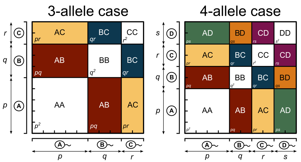
Yes, but the equation becomes extended.
For three alleles (A₁, A₂, A₃) with frequencies p, q, and r:
The expanded equation is p² + q² + r² + 2pq + 2pr + 2qr = 1.
Each term represents the expected frequency of a specific genotype.
Although less commonly tested, this form of the principle is useful in studying loci with multiple alleles, such as the ABO blood group system in humans.
Random mating ensures that alleles combine purely by chance, so genotype frequencies reflect allele frequencies accurately.
If mating is non-random, such as through inbreeding or assortative mating, homozygous genotypes become more common and heterozygotes less common.
This shifts genotype frequencies away from Hardy–Weinberg predictions, even if allele frequencies remain unchanged, thus violating equilibrium conditions.
Environmental changes can act as selective pressures that alter allele frequencies.
For example:
A change in climate may favour alleles for heat tolerance.
The appearance of a new predator may select for camouflage alleles.
When such pressures consistently favour or disadvantage certain alleles, natural selection occurs, causing deviations from Hardy–Weinberg equilibrium and leading to evolutionary adaptation within the population.
