Understanding Gradients and Intercepts

In A-Level Chemistry, graphs are powerful tools for analysing experimental data and determining relationships between variables. By carefully measuring gradients and intercepts, chemists can extract meaningful quantities such as rate constants, equilibrium constants, and enthalpy changes. Mastering these skills ensures accurate interpretation of results and supports valid conclusions based on evidence.

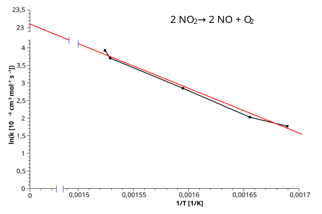
Arrhenius plot showing ln k versus 1/T with a clear straight-line fit. The gradient (−Ea/R) and y-intercept (ln A) can be read directly to obtain kinetic parameters. The axis break highlights the intercept region for clarity. Source

Importance of Linear Relationships

Many chemical relationships can be expressed as linear equations, which take the general form:

Linearising non-linear relationships allows experimental data to be interpreted more easily. For example, in rate or thermodynamic studies, transforming equations to a linear form enables determination of constants through graphical methods.

Selecting Appropriate Axes

Choosing suitable axes is crucial to ensure accurate measurement of gradients and intercepts.

• The independent variable should be plotted on the x-axis, as it is the quantity the experimenter controls.

• The dependent variable should be plotted on the y-axis, as it changes in response.

• Both axes must include units and consistent scaling to maintain proportional spacing between data points.

• Where relationships involve logarithmic or reciprocal values, appropriate transformations (e.g., plotting 1/[A] or ln p) should be made before graphing.

Proper axis selection ensures that the resulting plot correctly represents the underlying mathematical relationship.

Measuring the Gradient

The gradient represents the rate of change of one variable with respect to another. It quantifies how much the dependent variable changes for each unit change in the independent variable.

To obtain an accurate gradient:

• Draw the line of best fit that represents the overall trend of the data.

• Mark two well-separated points on the line (not necessarily data points).

• Read coordinates accurately, including units and decimal precision.

• Calculate Δy and Δx, ensuring consistent units.

Large, well-separated points minimise percentage error and improve reliability of the calculated gradient.

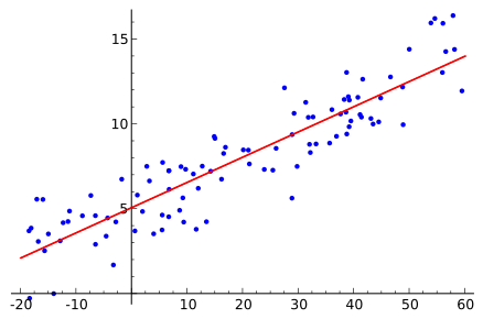
Scatter plot with a straight regression line. The gradient (rise over run) is taken from any convenient triangle on the line, and the intercept is the point where the line crosses the y-axis. Axes are clearly labelled to emphasise units. Source

Determining the Intercept

The intercept is the value of the dependent variable when the independent variable equals zero. It represents the point where the line crosses the y-axis.

In experimental chemistry, intercepts can reveal important constants:

• In Arrhenius plots (ln k vs 1/T), the intercept corresponds to ln A, the natural logarithm of the pre-exponential factor.

• In Beer–Lambert law graphs (A vs c), the intercept ideally equals zero if no systematic error or instrument offset exists.

• In calibration curves, the intercept indicates any baseline offset or background signal.

Accurate determination of the intercept allows meaningful comparisons between theoretical and experimental constants.

Using Graphical Methods to Determine Constants

Experimental data are often transformed into linear forms to allow constants to be derived from the gradient or intercept. Examples include:

• Rate equations: For first-order reactions, plotting ln [A] against time gives a straight line with gradient = −k.

• Arrhenius equation: Plotting ln k against 1/T yields a gradient = −Ea/R and intercept = ln A.

• Gas laws: A plot of P versus T (for constant volume) gives gradient = nR/V.

In each case, accurate graphical analysis ensures correct determination of key physical or chemical parameters.

Ensuring Accuracy and Precision in Measurement

To achieve reliable graphical results:

• Always use axes that cover at least two-thirds of the available graph paper to reduce reading uncertainty.

• Label axes clearly with quantities and units.

• Avoid joining data points directly; instead, draw a best-fit line using a ruler or software.

• When estimating the gradient, use a large triangle between two points on the line to reduce rounding and measurement error.

• Maintain consistent significant figures that reflect the precision of the experimental data.

Accurate plotting and measurement contribute directly to the validity and reproducibility of analytical results.

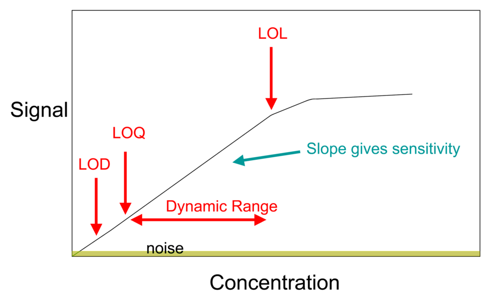
Calibration curve with a straight-line fit suitable for obtaining gradient and y-intercept from analytical data. This version additionally labels LOD, LOQ, and linearity limits; these features exceed the syllabus scope but the straight-line elements remain directly applicable. Source

Recognising and Reducing Errors

Common sources of error when measuring gradients and intercepts include:

• Poorly scaled axes, leading to distorted slopes.

• Incorrectly drawn best-fit lines, especially if biased towards certain data points.

• Inconsistent unit conversions, causing gradient misinterpretation.

• Limited data spread, which increases uncertainty in slope measurement.

• Graph reading errors, such as parallax or rounding mistakes.

Reducing these errors involves careful plotting, consistent units, and repeated analysis. Modern data software can also be used to minimise human error while retaining understanding of manual methods.

Using Linearised Plots Effectively

Not all relationships are naturally linear. In such cases, linearisation helps simplify complex expressions. For instance:

• The Arrhenius equation, k = A e^(−Ea/RT), becomes ln k = −Ea/R (1/T) + ln A when linearised.

• The first-order rate law, [A] = [A]₀ e^(−kt), becomes ln [A] = −kt + ln [A]₀.

By transforming these relationships into straight-line form, chemists can determine constants like activation energy (Ea) or rate constant (k) from the gradient and intercept of the plot.

Recording and Reporting Graphical Results

After measuring the gradient and intercept:

• Express the gradient with appropriate units derived from the variables’ quantities (e.g., mol dm⁻³ s⁻¹ per K).

• Record the intercept value with matching significant figures to ensure consistency.

• Clearly annotate graphs with any lines used to determine Δx and Δy.

• Include a short note describing how constants were obtained and what they represent chemically.

Proper recording practices ensure clarity in data analysis and support transparent evaluation during assessment.

Application in Experimental Evaluation

Evaluating the accuracy of a graph involves checking whether the gradient and intercept align with expected theoretical values. Deviations may indicate:

• Measurement or systematic errors.

• Incorrect unit conversions.

• Experimental design flaws affecting precision.

Through accurate determination of gradients and intercepts, students demonstrate their ability to link quantitative data to chemical principles, fulfilling the OCR requirement to “measure gradients and intercepts accurately from linearised plots to determine relationships and constants from experimental data.”