
OCR Specification focus:
‘Interpret and sketch graphs of transverse and longitudinal waves.’
Graphing waves allows physicists to visualise wave motion, understand phase relationships, and interpret spatial and temporal variations in displacement. Mastering wave graphs is essential for analysing behaviour, comparing wave types, and applying key equations in quantitative problems.
Understanding Wave Graphs
Graphical representation of waves provides a snapshot of how displacement varies either with time or with distance. Each type of graph conveys different but complementary information about wave behaviour.
Types of Wave Graphs
Displacement–Distance Graphs: Show the shape of the wave along a medium at a single instant in time.
Displacement–Time Graphs: Show how one point on the wave oscillates over time.
Both are indispensable tools for interpreting wave properties such as wavelength, amplitude, period, and frequency.
Key Quantities Represented on Graphs
Amplitude and Displacement
Amplitude (A): The maximum displacement of a particle from its equilibrium position.
Displacement (x): The distance and direction of a point on the wave from its rest position at a given time.
On both graph types, the peak and trough (for transverse waves) or compression and rarefaction (for longitudinal waves) indicate the maximum displacements. The amplitude is measured from the equilibrium line to a crest or trough.
Amplitude is linked directly to energy — higher amplitude means greater energy transfer.
Wavelength and Period
Wavelength (λ): The distance between identical points on adjacent waves (e.g., crest to crest).
Period (T): The time taken for one complete oscillation or wave cycle.
In a displacement–distance graph, wavelength is the horizontal distance between successive crests or troughs.
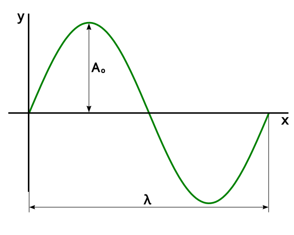
A labeled transverse wave showing amplitude (maximum displacement from equilibrium) and wavelength (distance between equivalent points such as crest to crest). Such displacement–distance graphs provide a spatial snapshot of the waveform at one instant. The simple layout matches OCR expectations without extra, off-syllabus detail. Source.
In a displacement–time graph, period is the horizontal time interval between identical displacement points in successive cycles.
Frequency and Phase Difference
Frequency (f): The number of complete cycles passing a point per second (measured in hertz, Hz).
Phase Difference (ϕ): The difference in phase between two points on a wave, indicating how far one is ahead or behind another in its cycle.
The frequency can be determined from the period using:
EQUATION
—-----------------------------------------------------------------
Frequency–Period Relationship (f) = 1 / T
f = frequency (Hz)
T = period (s)
—-----------------------------------------------------------------
On a displacement–time graph, points that reach maximum displacement at different times show phase differences. One full cycle equals a phase change of 360° or 2π radians.
Graphing Transverse and Longitudinal Waves
Transverse Waves
In transverse waves, oscillations are perpendicular to the direction of energy transfer. Examples include waves on strings and electromagnetic waves. When graphed as displacement–distance, the shape resembles a sine curve or cosine curve, depending on the phase.
Key features to label:
Crests: points of maximum positive displacement
Troughs: points of maximum negative displacement
Equilibrium line: the rest position
Wavelength (λ): distance between consecutive crests or troughs
In a displacement–time graph, a single particle’s motion traces a sinusoidal oscillation as it moves up and down over time.
Longitudinal Waves
For longitudinal waves, oscillations are parallel to the direction of energy transfer, such as in sound waves. These are visualised using compressions (regions of high pressure) and rarefactions (regions of low pressure).
A displacement–distance graph shows alternating regions of compression and rarefaction.
The distance between two consecutive compressions (or rarefactions) equals one wavelength.
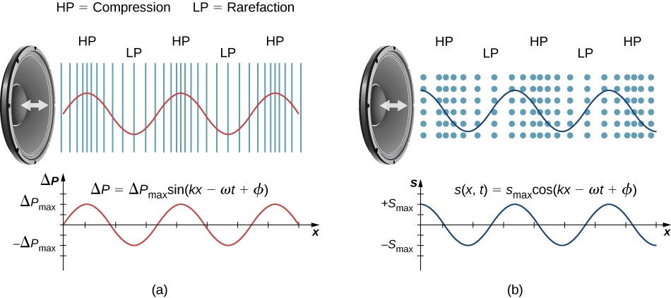
A longitudinal sound wave produced by a speaker, showing compressions and rarefactions in the air. The accompanying graphs plot pressure and particle displacement against distance, clarifying what a displacement–distance graph represents for longitudinal waves. Note: the panel also references pressure graphs; this is slightly beyond the minimal OCR wording but helpful for reading longitudinal plots. Source.
In displacement–time graphs, each particle vibrates back and forth about its equilibrium, similar in appearance to that of a transverse wave graph for one point.
Relationships Shown in Wave Graphs
Wave Speed and Wavelength
EQUATION
—-----------------------------------------------------------------
Wave Speed (v) = f × λ
v = wave speed (m/s)
f = frequency (Hz)
λ = wavelength (m)
—-----------------------------------------------------------------
Although wave speed is not directly shown on a static graph, it can be inferred from how wavelength and period relate — longer wavelengths or shorter periods correspond to higher speeds for a given frequency.
Phase and Position Relationships
At any instant, points along a displacement–distance graph can be at different phases.
For instance:
Two points separated by one full wavelength are in phase (phase difference 0°).
Points separated by half a wavelength are in antiphase (phase difference 180°).
This concept helps explain phenomena such as interference and standing waves, which rely on understanding how phase varies spatially.
Practical Interpretation Skills
To interpret wave graphs effectively, students must:
Identify axes: Distinguish whether the horizontal axis represents time (s) or distance (m).
Read amplitude and wavelength accurately: Use scale markings to measure quantities precisely.
Relate graphs to physical motion: For a particle at a point, determine its velocity and acceleration from the slope of displacement–time graphs.
Sketch graphs from descriptions: Be able to draw the expected form when given amplitude, wavelength, or frequency information.
Distinguish between stationary and progressive waves: In progressive waves, the pattern moves; in stationary waves, nodes and antinodes remain fixed.
These interpretive skills bridge visual understanding with the mathematical description of waves.
Graphing Techniques and Conventions
Axis Labelling and Units
Always label axes clearly:
Displacement (m) on the vertical axis.
Distance (m) or Time (s) on the horizontal axis, depending on the graph type.
Use consistent units and scales to ensure proportionality and clarity.
Sketching a Sinusoidal Wave
When sketching a transverse wave:
Begin at equilibrium for a sine representation or at maximum amplitude for a cosine representation.
Include one or more full cycles for clarity.
Indicate direction of travel with an arrow if required.
For longitudinal waves, represent compressions as vertical bars or regions of high density, spaced by one wavelength apart, and label rarefactions between them.
Interpreting Gradients and Motion
In displacement–time graphs:
The gradient at any point represents the velocity of the particle (rate of change of displacement).
The steeper the gradient, the greater the particle speed at that moment.
In displacement–distance graphs:The waveform shape represents an instantaneous position profile, not particle trajectories.
Summary of Graphing Insights
Graphing waves allows the extraction of critical relationships among displacement, time, and distance. Correctly interpreted, these graphs reveal amplitude, wavelength, period, frequency, and phase — essential characteristics for any analysis of wave behaviour in both transverse and longitudinal systems.
Practice Questions
Question 1 (2 marks)
The diagram below shows a displacement–distance graph of a transverse wave at a particular instant.
Explain what physical quantities can be determined directly from this graph and describe how they can be measured.
Mark scheme:
1 mark for identifying that wavelength can be determined as the distance between successive crests or troughs.
1 mark for identifying that amplitude can be measured as the maximum displacement from the equilibrium position.
Question 2 (5 marks)
A student sketches a displacement–time graph for a point on a progressive transverse wave. The wave has a period of 0.02 s and an amplitude of 4.0 mm.
(a) Describe how the shape and features of this displacement–time graph would appear, including any relevant quantities that can be determined from it.
(b) Explain how this graph would differ from a displacement–distance graph of the same wave at a single instant.
Mark scheme:
(a) 1 mark for describing that the graph would be a sinusoidal curve showing periodic oscillations about an equilibrium line.
(a) 1 mark for stating that the amplitude is 4.0 mm (maximum displacement).
(a) 1 mark for identifying that the period is 0.02 s, corresponding to the time between two identical points on consecutive cycles.
(b) 1 mark for explaining that the displacement–time graph shows how one point oscillates over time, while the displacement–distance graph shows wave shape along the medium at one instant.
(b) 1 mark for noting that on the displacement–distance graph, the wavelength can be determined, whereas on the displacement–time graph, the period can be determined.
FAQ
A displacement–time graph shows how a single point oscillates with time, so all particles follow the same pattern but at different times. A displacement–distance graph, however, shows the shape of the wave at one instant across space.
To distinguish:
If the horizontal axis has units of seconds (s), it’s a displacement–time graph.
If it has units of metres (m), it’s a displacement–distance graph.
The time graph repeats with a period (T), while the distance graph repeats with a wavelength (λ).
In a progressive wave, energy and phase travel through the medium. Over time, the displacement–distance pattern appears to shift in the direction of energy transfer.
For example:
A rightward-moving wave will have its crests and troughs moving right.
The phase at a given position changes continually, so the graph must be redrawn for each instant to represent the moving pattern.
The graph retains the same sinusoidal shape and period, as frequency and period are unchanged.
However:
The vertical scale of the oscillation increases because the maximum displacement (amplitude) is larger.
This means each crest and trough extends further above and below the equilibrium line, indicating higher energy transmission without affecting timing.
Phase difference describes how far apart two oscillations are within their cycles. On graphs, it’s represented by horizontal separation between identical points on different waves.
For instance:
Two waves that reach their peaks at the same position or time are in phase.
If one reaches its peak when the other reaches its trough, they are in antiphase (180° apart).
The greater the horizontal offset, the larger the phase difference.
A displacement–distance graph represents positions of points at a single instant, not their motion through time. The slope of this graph doesn’t correspond to particle velocity.
To find velocity, a displacement–time graph is needed:
The gradient at any point gives the instantaneous velocity.
Steeper gradients indicate faster movement.
Only time-based data can show how displacement changes per second, which defines velocity.
