
OCR Specification focus:
‘Distinguish instantaneous and average quantities; calculate from data, including gradients and areas on motion graphs.’
Understanding the distinction between instantaneous and average quantities is fundamental to analysing motion accurately. These concepts underpin the interpretation of motion graphs and practical experimental measurements.
Instantaneous and Average Quantities
Instantaneous Quantities
Instantaneous quantities describe a value at a specific moment in time rather than over a period. They provide a snapshot of motion and are particularly useful when analysing changing movement.
Instantaneous Speed: The rate of change of distance with respect to time at a specific instant.
Instantaneous Velocity: The rate of change of displacement with respect to time at a specific instant, including direction.
Instantaneous Acceleration: The rate of change of velocity with respect to time at a specific instant.
Instantaneous quantities are typically determined from gradients of tangents drawn to curves on motion graphs.
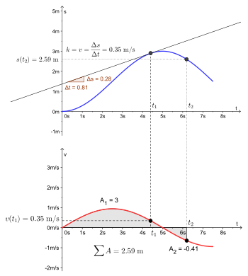
A clean diagram showing how a tangent to the displacement–time curve gives the instantaneous velocity, with the corresponding point located on the velocity–time graph. This directly supports using gradients for instantaneous quantities. Labels are minimal and focused on the s–t and v–t relationship. Source.
For example, on a displacement–time graph, the gradient of a tangent gives the instantaneous velocity. Similarly, on a velocity–time graph, the gradient of a tangent gives the instantaneous acceleration.
Because they represent conditions at one precise time, instantaneous quantities are ideal for analysing motion where speed or acceleration varies continuously, such as an object in free fall or a car accelerating.
Average Quantities
Average quantities summarise motion over a finite interval of time. They are often simpler to calculate but provide less detailed information about variations within that period.
Average Speed: The total distance travelled divided by the total time taken.
Average Velocity: The total displacement divided by the total time taken.
Average Acceleration: The change in velocity divided by the time taken for that change to occur.
Average quantities are calculated directly from measurements or data, particularly when experimental tools only capture values over intervals rather than at single instants. For example, average velocity can be found by dividing total displacement by elapsed time.
A short sentence about their significance: Average quantities provide useful comparisons between different motions or experimental runs where precise instantaneous data may not be available.
Measuring and Calculating Instantaneous and Average Values
Using Gradients on Motion Graphs
Graphs are central to determining motion quantities. The gradient (slope) of a graph represents a rate of change — the basis for connecting physical quantities in kinematics.
On a displacement–time graph:
The gradient gives the velocity.
A straight line indicates constant velocity, while a curve shows changing velocity.
On a velocity–time graph:
The gradient gives the acceleration.
A horizontal line indicates constant velocity (zero acceleration).
A sloped line represents uniform acceleration.
To find an instantaneous value from such a graph:
Draw a tangent to the curve at the specific point of interest.
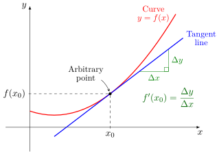
A simple, labelled diagram of a tangent to a curve highlighting the slope at a point. This underpins the method for reading instantaneous velocity or acceleration from motion graphs. Extra mathematical symbols are minimal; the focus is solely on the tangent concept. Source.
Calculate the gradient of that tangent using the rise over run method.
The resulting value is the instantaneous speed, velocity, or acceleration, depending on the graph type.
EQUATION
—-----------------------------------------------------------------
Gradient Relationship (General) = Change in y / Change in x
Change in y = Difference in the dependent variable (e.g. displacement or velocity)
Change in x = Difference in the independent variable (usually time, s)
—-----------------------------------------------------------------
This method is key to distinguishing between average and instantaneous quantities: an average gradient considers the entire interval, while an instantaneous gradient uses only the tangent at one point.
Using Areas on Motion Graphs
In addition to gradients, areas under curves provide information about accumulated quantities over time.
On a velocity–time graph, the area under the curve gives the displacement.
On an acceleration–time graph, the area under the curve gives the change in velocity.
To find average velocity from a velocity–time graph:
Divide the total area under the curve (representing total displacement) by the total time.
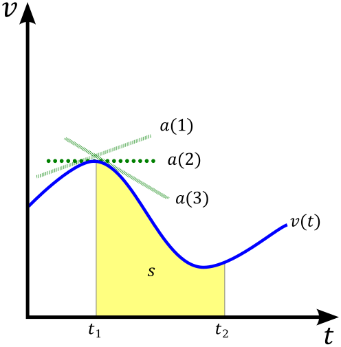
An annotated velocity–time graph indicating slope for acceleration and shaded area for displacement. This figure supports average and instantaneous reasoning: local slope for instantaneous acceleration versus total shaded area for displacement over an interval. The content is tightly aligned to OCR requirements without extraneous detail. Source.
This links graphical representation directly with physical interpretation, enabling both instantaneous and average quantities to be extracted from data.
EQUATION
—-----------------------------------------------------------------
Average Velocity (v̄) = Total Displacement (Δs) / Total Time (Δt)
Δs = Total displacement in metres (m)
Δt = Total time interval in seconds (s)
—-----------------------------------------------------------------
Between these calculations, a clear distinction emerges: instantaneous values are local (from tangents), whereas average values are global (from intervals).
Practical Measurement of Instantaneous and Average Values
In experiments, capturing motion data with high precision often involves data loggers, light gates, or video analysis systems. These tools enable accurate timing and distance measurements.
Average velocity may be measured using:
Two light gates separated by a known distance, recording the total time between interruptions.
Manual timing with a stopwatch for larger intervals (less accurate).
Instantaneous velocity can be found by:
Using a single light gate that measures how long an object blocks a beam, combined with the known length of the object.
Employing motion sensors or data loggers that sample positions at very short time intervals.
By reducing the measurement interval, instantaneous values can be approximated more closely. In digital systems, a high sampling rate produces near-instantaneous data by recording positions or velocities many times per second.
Interpreting Experimental Data
When analysing motion data:
Plot displacement–time and velocity–time graphs.
Use average gradients for general trends and tangent gradients for instantaneous values.
Estimate areas under curves using counting squares, geometric shapes, or numerical integration for non-linear data.
Precision improves when:
Time intervals are small.
Measurement devices have high temporal resolution.
Graphs are plotted with sufficient scale and clarity to identify gradients accurately.
The ability to calculate and distinguish between instantaneous and average quantities allows physicists to describe motion comprehensively, interpret data effectively, and connect mathematical models to physical phenomena in the study of kinematics.
Practice Questions
Question 1 (2 marks)
A car travels along a straight road. At one moment, its velocity changes from 12 m s⁻¹ to 18 m s⁻¹ in 3.0 s.
(a) Calculate the average acceleration of the car during this time interval.
(b) State how the instantaneous acceleration at a point in time differs from the average acceleration over a period.
Mark Scheme for Question 1
(a) Average acceleration = (change in velocity) / (time taken)
= (18 – 12) / 3.0 = 2.0 m s⁻²
• Correct substitution and working (1 mark)
• Correct final answer with unit (1 mark)
(b) Instantaneous acceleration refers to the acceleration at a specific moment, whereas average acceleration is over a time interval.
• Distinction made between “at an instant” and “over a time interval” (1 mark, if part (b) asked independently)
Question 2 (5 marks)
The graph below shows how the velocity of a cyclist changes with time during a short journey.
The graph is a curve starting at 0 m s⁻¹ at t = 0, increasing steeply to 8 m s⁻¹ at 4 s, then flattening slightly to 10 m s⁻¹ at 6 s.
(a) Describe how the instantaneous acceleration of the cyclist changes between t = 0 s and t = 6 s.
(b) Explain how you would determine the instantaneous acceleration of the cyclist at t = 2 s from the graph.
(c) The cyclist travels for a total of 6 s. Describe how to estimate the average velocity of the cyclist during this period using the graph, and outline one reason why the estimated value may differ from the instantaneous velocity at t = 3 s.
Mark Scheme for Question 2
(a)
• Acceleration is large initially because the gradient of the velocity–time graph is steep (1 mark)
• Acceleration decreases as the curve becomes less steep (1 mark)
(b)
• Draw a tangent to the curve at t = 2 s (1 mark)
• Determine the gradient of that tangent (Δv/Δt) to find the instantaneous acceleration (1 mark)
(c)
• Estimate the area under the velocity–time graph to find total displacement (1 mark)
• Divide displacement by total time to obtain average velocity (1 mark)
• Difference arises because the average velocity represents motion over the whole period, while instantaneous velocity applies to a single point (1 mark)
FAQ
The main source of error is drawing the tangent inaccurately. Small changes in the tangent’s slope can lead to large variations in the calculated velocity.
Other common issues include:
Poor graph scale or coarse time intervals, reducing precision.
Parallax error when reading plotted points.
Using a ruler that doesn’t align exactly with the intended tangent point.
To reduce error, ensure the graph has a clear scale, large plotting area, and tangents are drawn with fine accuracy using smooth curves.
Light gates measure time electronically and respond almost instantly when the beam is interrupted, removing human reaction delay.
When a moving object of known length passes through the beam, the gate measures the blockage duration, from which instantaneous speed can be calculated as:
Speed = length of object / time beam blocked
In contrast, stopwatches rely on manual timing, introducing variability and typically reducing precision to ±0.1 s or worse.
No, because every measurement device has a finite response time. Even very fast sensors sample data over a small, but non-zero, interval.
However, instantaneous quantities can be approximated closely by:
Using high-speed sensors or data loggers with microsecond sampling.
Ensuring smooth, continuous motion to limit rapid changes during sampling.
Physicists treat these approximations as effectively instantaneous if the time interval is negligible compared to the motion’s total duration.
Computer systems, such as video tracking software or motion sensors, record position data at fixed sampling intervals and display displacement–time and velocity–time graphs automatically.
From this data:
Average values are derived from total changes over longer periods.
Instantaneous values are calculated using differential methods, often by estimating gradients between successive data points.
Such tools improve precision and allow rapid comparison between instantaneous and average results in experimental investigations.
The area under a velocity–time graph integrates all changes in velocity continuously, accounting for acceleration and deceleration.
Manual methods, such as using metre rulers or tapes, may ignore small variations in speed or path curvature. The graphical area method captures these variations automatically if the velocity data is accurate.
For irregular curves, software or counting-square methods provide better estimates of total displacement than physical distance tracking, which is prone to cumulative measurement error.
